$$$$

21  Fundamental Theorems

We’ve already made great progress in the theory of integrating vector valued functions by converting circulation/work integrals into

21.1 The Fundamental Theorem of the Gradient

Theorem 21.1 (Fundamental Theorem of the Gradient) Let $f$ be a scalar function and $\overrightarrow{F}=\mathrm{\nabla }f$ its gradient. Then if $C$ is a curve from $p$ to $q$, the line integral of $F$ can be evaluated as $${\int }_C\mathrm{\nabla }f\cdot d\overrightarrow{s}=f(q)-f(p)$$

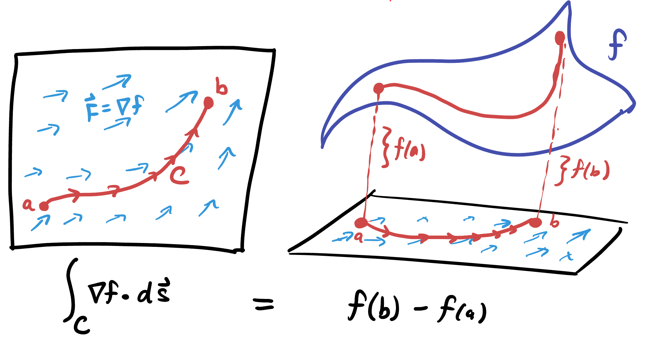
This is a direct analog of the 1 dimensional fundamental theorem of calculus which tells us we can evaluate an integral by finding an antiderivative and evaluating at the endpoints - we’ve just generalized to replace the interval $[a,b]$ along the real line with a curve $C$, and the derivative of a function with the gradient.

In fact, the proof of the original fundamental theorem generalizes directly to this case as well, as we saw in class: $\mathrm{\nabla }f\cdot c^{\prime }$ is the directional derivative of $f$ in the direction of the curve $c$, and integrating this over its length adds up all these infinitesimal changes in height to get the net change in height: the value of $f$ at the endpoint minus the value of $f$ at the start.

There is one subtlety in higher dimensions which did not occur in the one dimensional case. For 1 variable functions every continuous function has an antiderivative, so we can always apply the fundamental theorem if we can find it. But for vector fields we’ve already seen that not every vector field has a potential: indeed, a necessary condition for a continuous vector field to have a potential is that its curl is zero. (This is a useful concept, so its nice to have a single word for it: recall we call such vector fields conservative).

Definition 21.1 A vector field $F$ is called conservative if it has an antiderivative with respect to the gradient. Any such antiderivative $f$ with $\mathrm{\nabla }f=F$ is called a potential for $F$. If $F$ is continuous and defined everywhere, then $F$ is conservative if and only if its curl is zero.

The fundamental theorem for the gradient makes it easy to evaluate integrals if you can find the potential. But it also has some interesting theoretical consequences:

Corollary 21.1 (Path Independence) If $\overrightarrow{F}$ is a conservative vector field then the value of its line integral along a curve $C$ between points $p$ and $q$ is independent of the path.

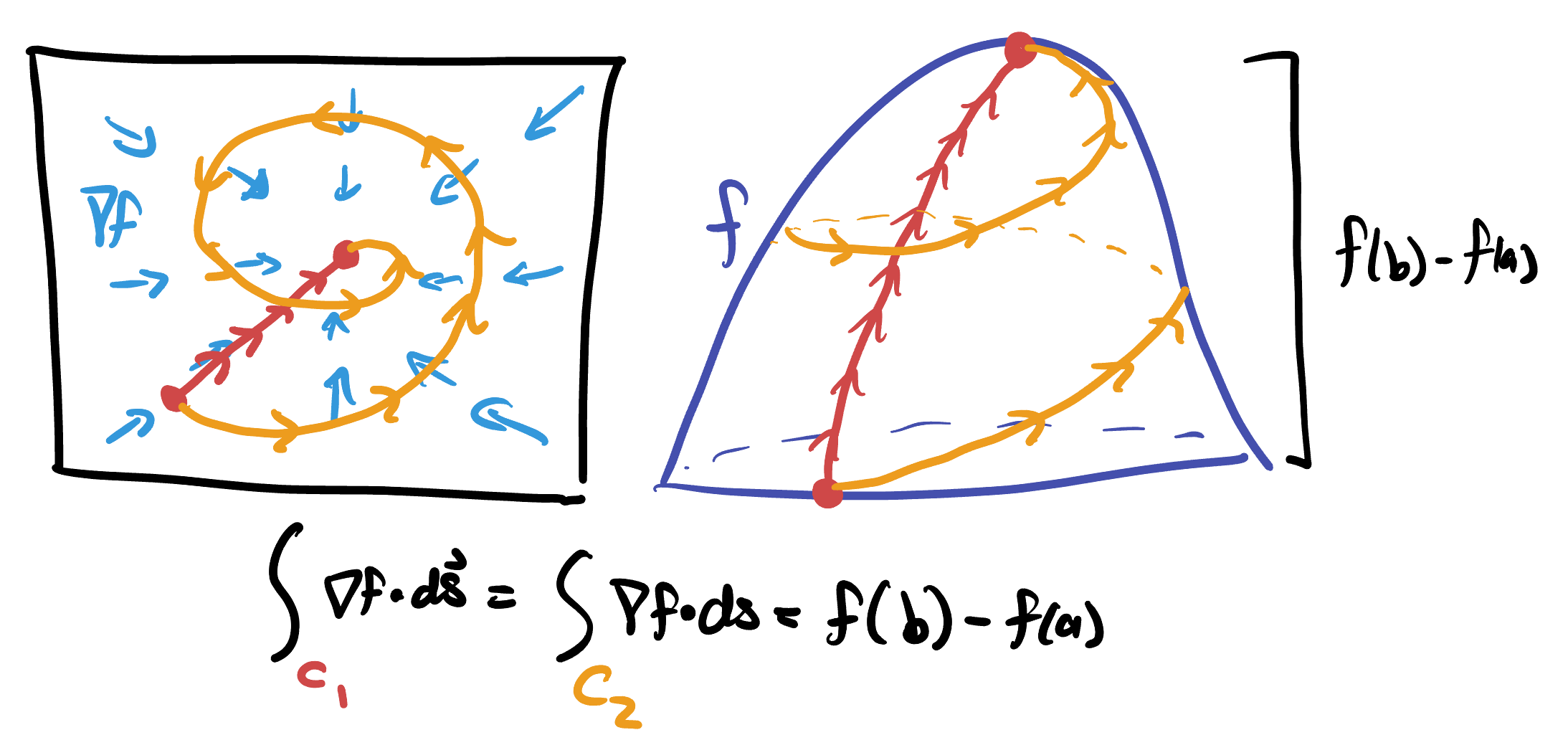
This is a rather striking property at first - it means for these vector fields it doesn’t even matter what path we integrate them along: so long as the paths start and end at the same point the circulation integral will have the same value!

Example 21.1 Compute the line integral of $(3+4x{y}^2)\hspace{0.17em}i+4x^{2}y\hspace{0.17em}j$ along the arc of the unit circle joining $(1,0)$ to $(0,1)$.

Example 21.2 Integrate the circulation of $F=⟨x+1,y^2-2y-1⟩$ along the curve $c(t)=⟨t^2-2t,t+1⟩$ for $t\in [0,2]$.

Corollary 21.2 (Integrating around Closed Curves) Let $C$ be a closed curve and $\overrightarrow{F}$ be a conservative vector field. Then $${\oint }_C\overrightarrow{F}\cdot d\overrightarrow{s}=0$$

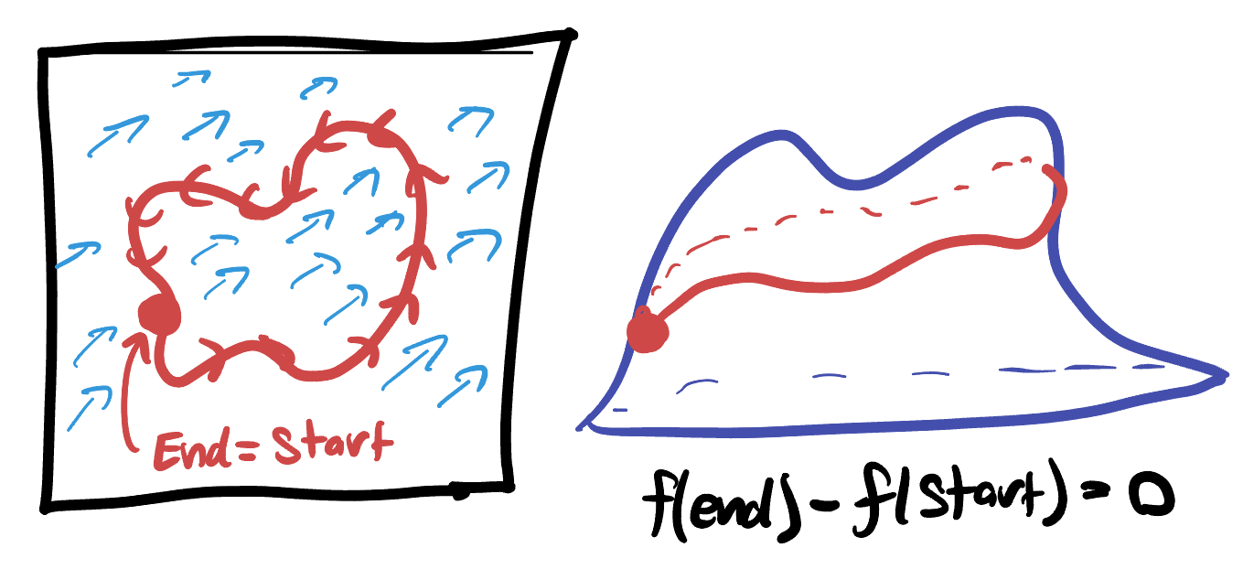
Like above, the proof is simple: since $\overrightarrow{F}$ is conservative there is a potential $\mathrm{\nabla }f=\overrightarrow{F}$ and so we can apply the fundamental theorem. But since $C$ is a closed curve, its endpoint equals its start point, so $f(\mathrm{end})=f(\mathrm{start})$ and their difference is zero. This is quite useful as it lets us often evaluate difficult looking integrals with almost no work at all.

Example 21.3 Compute the integral of $\overrightarrow{F}=⟨x^4{y}^5\hspace{0.17em},x^5{y}^4\hspace{0.17em}⟩$ $ around the closed curve $c(t)=⟨1+\cos (2t)+\sin (t),{\sin }^2(t)+\cos (t)-1⟩$ for $t\in [0,2\pi ]$.

Solution: Since the curve is closed, we check if the vector field is conservative by computing its curl: $$\mathrm{\nabla }\times \overrightarrow{F}==0$$ Since $F$ is defined everywhere and $\mathrm{\nabla }\times F=0$, we know that a potential exists, and so the integral around any closed loop is zero: we’re done!

Of course this doesn’t work if the curl turns out to be nonzero, as then the vector field is not conservative, and there exists no potential for which to apply the fundamental theorem. In such cases we can always go back and just evaluate the line integral with our original method, finding $F(c(t))\cdot c^{\prime }(t)$ and integrating along the curve. But there’s also another fundamental theorem that can come to our aid, discussed below.

21.2 The Fundamental Theorem of the Curl

Recall that we called an antiderivative for the curl a vector potential: given a field $F$ a vector potential is another field $A$ such that $\mathrm{\nabla }\times A=F$. This type of derivative comes with its own fundamental theorem as well, now relating double integrals to single integrals. To write it in language reminiscent of the original fundamental theorem, one might say

Let $F$ be a field and $A$ be a vector potential for $F$. Then if $D$ is a region in the plane whose boundary is the closed curve $C$, one has $${\iint }_{D}FdS={\oint }_{C}A\cdot ds$$

That is - taking hte antiderivative for curl removes one of the integrals! This theorem is more commonly stated without giving a separate name to the vector potential $A$, but instead writing out the curl explicitly:

Theorem 21.2 (2D Fundamental Theorem of the Curl (Green’s)) Let $D$ be a region in the plane whose boundary is the closed curve $C$ and $F$ a vector field. Then $${\iint }_D\mathrm{\nabla }\times FdA={\oint }_{C}F\cdot d\overrightarrow{s}$$

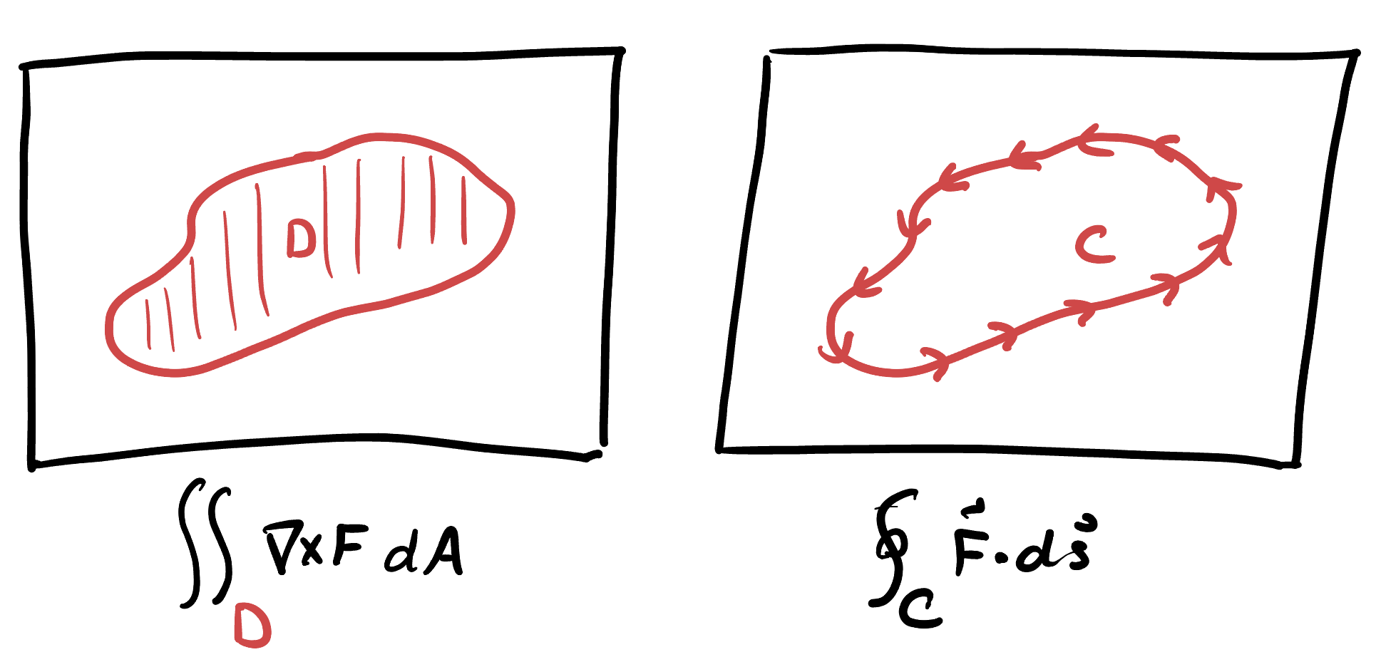
In two dimensions the curl is a scalar; indeed if $F=⟨P,Q⟩$ one might write this as $\mathrm{\nabla }\times F=Q_x-P_y$ giving the alternate form (same theorem, different symbols):

$${\iint }_D(Q_x-P_y)dA={\oint }_{C}Pdx+Qdy$$

This theorem is often mostly used in reverse: compute a line integral by turning it into a double integral! The reason is, that double integral is just the integral of a scalar function, and we’ve known how to do those for quite some time!

Example 21.4 Compute the line integral ${\oint }_{C}xdy-ydx$ around the circle of radius 3 centered at the origin, parameterized counterclockwise.

Solution: We could evaluate this integral directly by parameterizing $c(t)=(3\cos t,3\sin t)$. But the fundamental theorem says we could instead choose to take the curl and integrate over the interior of the circle $c$. Here $F=⟨-y,x⟩$ and $$\mathrm{\nabla }\times F={\partial }_{x}x+{\partial }_{y}y=2$$ Thus our integral becomes ${\iint }_{D}2dA$$ But integrating $2dA$ over a region just returns twice its area, and since our region is the circle of radius 2, this is $$2(\pi (2^2))=8\pi$$

Example 21.5 Compute the circulation integral $${\oint }_C{y}^{3}dx-x^{3}dy$$ For $C$ the circle of radius 2 about the origin, parameterized clockwise.

Solution: This line integral corresponds to the vector field $F=⟨y^3,-x^3⟩$, whose curl is $$\mathrm{\nabla }\times F=\left|\begin{array}{cc}{\partial }_x& {\partial }_y\\ y^3& -x^3\end{array}\right|=3y^2+3x^2=3(x^2+y^2)$$ Using the fundamental theorem we can integrate this over the interior of the circle of radius 2 instead of integrating $F$ along the boundary. This is easiest in polar coordinates where $3(x^2+y^2)=3r^2$ and $${\iint }_D\mathrm{\nabla }\times FdA={\int }_0^{2\pi }{\int }_0^{2}3r^{2}rdrd\theta =24\pi$$

This is particularly useful when the line integral is around a piecewise curve: instead of doing multiple line integrals and adding them all up, you can take the curl, and integrate that over the interior.

Example 21.6 Compute the circulation of $F=⟨y{e}^x,2e^x⟩$ around the boundary of the unit rectangle with vertices $(0,0),(1,0),(1,1)$ and $(0,1)$ parameterized counterclockwise starting at $(0,0)$.

There is a direct analog of this theorem in three dimensions, unchanged except for the fact that the curl is a vector field

Theorem 21.3 (3D Fundamental Theorem of the Curl (Stokes’s)) Let $C$ be a curve in 3D and $S$ be a surface whose boundary is $C$. Then if $F$ is a vector field $${\iint }_S\mathrm{\nabla }\times F\cdot d\overrightarrow{S}={\oint }_{C}F\cdot d\overrightarrow{s}$$

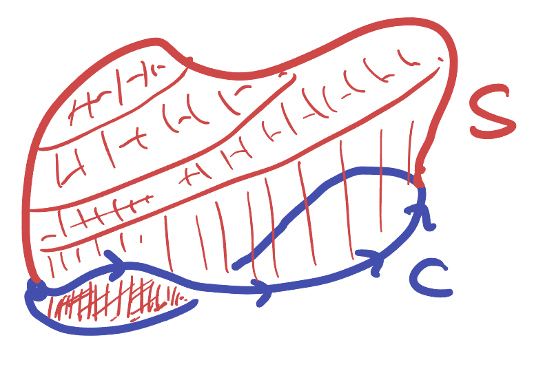
This can be used to compute circulation integrals around a 3D curve, by using a (hopefully simpler) surface that spans them. But it also makes for really easy calculations of integrals over a closed surface (like a sphere, with no boundary).

Example 21.7 Let $F$ be the vector field $F=⟨xy,y+1,z+x⟩$ and compute the flux of $\mathrm{\nabla }\times F$ through the sphere of radius $2$ centered at the origin.

Solution: Stokes theorem says that the integral of $\mathrm{\nabla }\times F$ over a surface $S$ is the same as the circulation around the boundary. But a sphere has no boundary! So there is no circulation around this boundary, and the integral is zero. This means our original double integral is also zero!

These sorts of computations are very useful in physics and electrical engineering, when working the electromagnetic field. For example, when there is a current $\overrightarrow{J}$ flowing and the electric field is not changing in time, the magnetic field satisfies $\mathrm{\nabla }\times B=J$, so the flux of current through a surface can be computed by integrating $\mathrm{\nabla }\times B$ on that surface, and then stokes theorem sayst this is the same as the integral of $B$ around the boundary. (We won’t dive into such applications here, but for those of you continuing onto electromagnetism this spring, this is where that class will pick up.)

21.3 The Fundamental Theorem of the Divergence

We’ve seen so far a pattern in generalizing the fundamental theorem of calculus to vector fields: given a type of derivative, we search for a corresponding notion of anti derivative, and using this antiderivative allows us to remove one integral: the derivative and antiderivative “cancel”. So perhaps it comes as no surprise that there is yet another fundamental theorem of calculus, this time paired with the divergence:

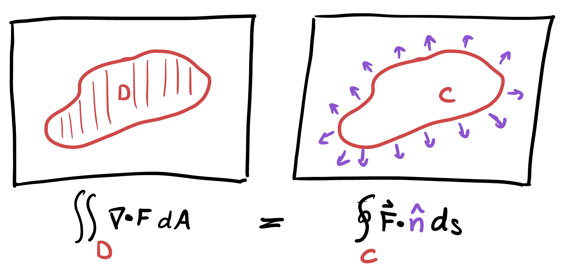
Theorem 21.4 (2D Fundamental Theorem of the Divergence) Let $F$ be a vector field in the plane and $\mathrm{\nabla }\cdot F$ be its divergence. Then given a closed curve $C$ bounding a region $D$ in the plane, the flux of $F$ through $C$ can be calculated by integrating its divergence over the interior $D$:

$${\oint }_{C}F\times d\overrightarrow{s}={\iint }_D\mathrm{\nabla }\cdot FdA$$

Recall that ${\oint }_{C}F\times d\overrightarrow{s}$ is shorthand for the flux integral, a dot product with the normal vector ${\oint }_{C}F\cdot nds$.

As written the theorem applies only to positively oriented curves: that is, those traversed counterclockwise. But its easy to use for negatively oriented curves if you remember that going the other way around the curve multiplies the line integral by $-1$.

This theorem also has a direct analog in three dimensions, replacing curve with surface and area with volume:

Theorem 21.5 (3D Fundamental Theorem of the Divergence (Gauss’)) Let $F$ be a 3D vector field and $\mathrm{\nabla }\cdot F$ its divergence. Then given a closed surface $S$ bounding a region $E$ in space, the flux of $F$ through $S$ can be calculated by integrating its divergence over the interior $E$:

$${\iint }_{S}F\cdot dS={\iiint }_E\mathrm{\nabla }\cdot FdV$$

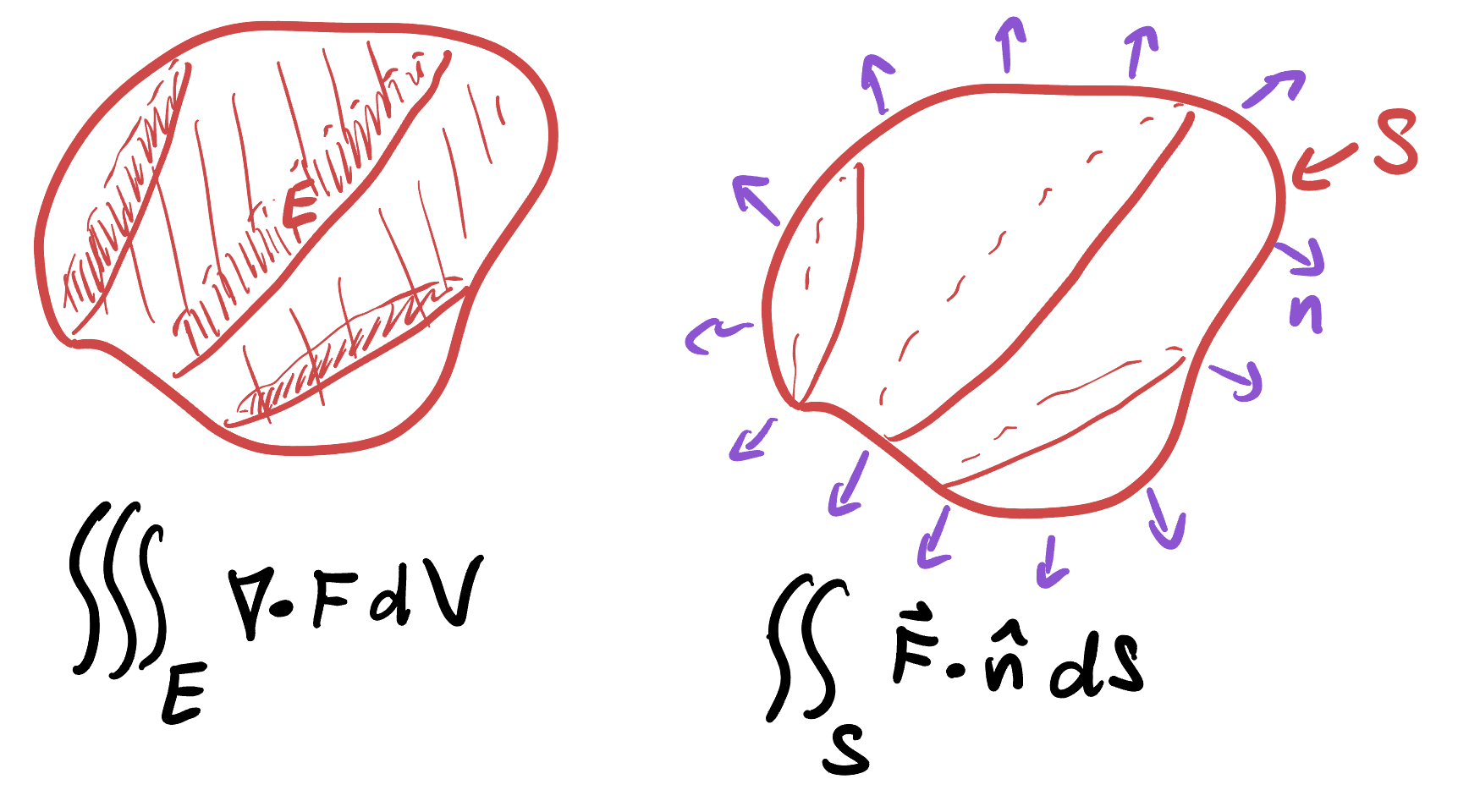
The intuition for this theorem is a little clearer than the case of curl, but essentially the same vibe: divergence measures how much a vector field spreads out at a point, and the flux integral captures how much it spreads out through a surface. The theorem just says that the net amount it spreads out through the curve/surface is the sum of the infinitesimal amounts it spreads out on the interior. This is again useful to take complicated line or surface integrals and replace them with easier double or triple integral of a scalar function.

Example 21.8 Use the divergence theorem to find the flux of $F=⟨x,y⟩$ through the sides of the triangle with vertices $(0,0)$, $(2,0)$ and $(2,1)$.

Example 21.9 Use the divergence theorem to calculuate the outward flux of $F=xy{e}^z\hspace{0.17em}i+x{y}^2{z}^3\hspace{0.17em}j-y{e}^z\hspace{0.17em}k$ through the box defined by the coordinate planes and $x=1$, $y=2$, $z=3$.

Often this triple integral can be easiest to compute by changing coordinates:

Example 21.10 Compute the flux of the vector field $F=⟨x,y,1⟩$ through the unit sphere.

Example 21.11 Compute the flux of $F=3x{y}^2\hspace{0.17em}i+x{e}^z\hspace{0.17em}j+z^3\hspace{0.17em}k$ through the surface of the solid cylinder bounded by $x^2+z^2=9$ and $x=0$,$x=3$.

21.4 The Bigger Picture

The original fundamental theorem of calculus in one variable emerged in the mid 1600s. Over the next two centuries the field matured and developed through various uses in multiple variables, and these new generalized versions of the fundamental theorem began to appear in rapid succession around the mid 1800s. While at the time each was discovered for its own bespoke use (often within electromagnetism) with our modern eyes we may take a look at the collection of fundamental theorems and see a hint of some deeper pattern:

$${\int }_a^b{f}^{\prime }dx=f(b)-f(a)$$ $${\int }_C\mathrm{\nabla }f\cdot d\overrightarrow{s}=f(b)-f(a)$$ $${\iint }_D\mathrm{\nabla }\times FdS={\oint }_{C}F\cdot d\overrightarrow{s}{\iint }_S\mathrm{\nabla }\times F\cdot d\overrightarrow{S}={\oint }_{C}F\cdot d\overrightarrow{s}$$ $${\iint }_D\mathrm{\nabla }\cdot FdS={\oint }_{C}F\cdot d\overrightarrow{s}{\iiint }_E\mathrm{\nabla }\cdot FdV={\iint }_{S}F\cdot d\overrightarrow{S}$$

On the left side of each of these we are integrating some derivative over a region (an interval, curve, surface, or volume). And on the right we are instead evaluating its antiderivative along the boundary of the original region. In the case of the interval or curve the boundary is just two points, so “evaluating on the boundary” is just subtracting their difference. On the higher dimensional regions the boundary is 1 or 2 dimensional, so “evaluating on the boundary” means doing a line or surface integral.

After noticing this pattern mathematicians went off in search of the correct framework to prove it in. One can already imagine several difficulties here in trying to unify the proofs of all these fundamental theorems: for one, curl behaves differently in dimension 2 (where its a scalar) and in dimension 3 (where its a vector). The correct language for combining discussions of vectors and scalars, as well as infinitesimal lengths, area elements and volume elements is called the theory of differential forms which developed over the mid-late 1800s. Differential forms are mathematical tools for working with

In 1889, Volterra discovered a fundamental theorem of calculus in this new language (often called the generalized Stokes Theorem)

Theorem 21.6 (Fundamental Theorem for Differential Forms) If $\omega$ is an $n-1$ differential form and $M$ is an $n$ dimensional region, then integrating $d\omega$ over $M$ is the same as integrating $\omega$ over the (n-1 dimensional) boundary of $M$. $${\iint }_{M}d\omega ={\int }_{\partial M}\omega$$

About a decade later Cartan realized in 1899 that the traditional language of vector calculus could all be rewritten within the theory of differential forms:

Theorem 21.7 (Differential Forms and Vector Calculus)  

• Zero forms are functions
• 1 forms are vector fields: and anything you can integrate over a curve.
• 2 forms measure infinitesimal areas, and anything you can integrate over a surface
• 3 forms measure infinitesimal volumes, and anything you can integrate over a 3D region

The exterior derivative of differential forms encodes familiar operations. In three dimensions:

• The derivative of a zero form is a 1 form: this corresponds to the gradient
• The derivative of a 1 form is a 2 form: this corresponds to the curl
• The derivative of a 2 form is a 3 form: this corresponds to the divergence

A few decades later, in 1917, the mathematician Edouard Goursat realized that all of the previously known fundamental theorems of calculus were special cases of the fundamental theorem for differential forms, essentially showing that the entire theory of vector calculus truly belongs as a special case of this new more general technology.