$$ \newcommand{\RR}{\mathbb{R}} \newcommand{\QQ}{\mathbb{Q}} \newcommand{\CC}{\mathbb{C}} \newcommand{\NN}{\mathbb{N}} \newcommand{\ZZ}{\mathbb{Z}} \newcommand{\EE}{\mathbb{E}} \newcommand{\HH}{\mathbb{H}} \newcommand{\SO}{\operatorname{SO}} \newcommand{\dist}{\operatorname{dist}} \newcommand{\length}{\operatorname{length}} \newcommand{\uppersum}[1]{{\textstyle\sum^+_{#1}}} \newcommand{\lowersum}[1]{{\textstyle\sum^-_{#1}}} \newcommand{\upperint}[1]{{\textstyle\smallint^+_{#1}}} \newcommand{\lowerint}[1]{{\textstyle\smallint^-_{#1}}} \newcommand{\rsum}[1]{{\textstyle\sum_{#1}}} \newcommand{\partitions}[1]{\mathcal{P}_{#1}} \newcommand{\erf}{\operatorname{erf}} \newcommand{\ihat}{\hat{\imath}} \newcommand{\jhat}{\hat{\jmath}} \newcommand{\khat}{\hat{k}} \newcommand{\pmat}[1]{\begin{pmatrix}#1\end{pmatrix}} \newcommand{\smat}[1]{\left(\begin{smallmatrix}#1\end{smallmatrix}\right)} $$

4 Shapes

(Relevant Sections of the Textbook: 12.5 Lines & Planes, and 12.6 Cylinders and Quadric Surfaces)

Lines and planes are given by linear equations: involving only the coordinate variables ($x,y,z$,etc), constants, and addition.

4.1 Lines

Definition 4.1 (Implicit Lines in $\RR^2$) An implicit line in the plane is an equation of the form \[ax+by=c\]. When $b\neq 0$ this can be put into $y=mx+b$ form as $y=-\frac{a}{b}x+\frac{c}{b}$.

Theorem 4.1 (Normal Direction to a Line) The implicit line $ax+by=c$ is orthogonal to the vector $\vec{n}=\langle a,b\rangle$.

How can we confirm this? Find two points along the line, subtract them to get their direction vector, then take the dot product of this with $\langle a,b\rangle$ - show its zero!

Finding the direction of a line by finding two points on it is tedious, so luckily once we know the above fact we don’t need to do this any more! Its easy to figure out the drection of an implicit line: if its orthogonal to $\langle a,b\rangle$, then it points in the direction $\langle -b,a\rangle$ (recall this vector is itself orthogonal to $\langle a,b\rangle$).

Definition 4.2 (Parametric Lines) A parametric line is a function of the form \[\ell(t)=p + t \vec{v}\] This passes through the point $p$ and is in the direction $\vec{v}$.

Open Fullscreen

Theorem 4.2 (Line Segment Between Two Points) If $\vec{p}$ and $\vec{q}$ are two points in space, the line segment between them can be parameterized by the following equation for $t\in[0,1]$. \[\begin{align*} \vec{\ell}(t)&=\vec{p}+t(\vec{q}-\vec{p})\\ &=(1-t)\vec{p}+t\vec{q} \end{align*}\]

4.2 Planes

Definition 4.3 (Implicit Planes I) A plane through the point $\vec{p}=\langle x_0,y_0,z_0\rangle$ with normal vector $\vec{n}=\langle a,b,c\rangle$ is determined by the scalar equation \[\vec{n}\cdot\left(\langle x,y,z\rangle-p\right)=0\] \[a(x-x_0)+b(y-y_0)+c(z-z_0)=0\]

Distributing and collecting all the constants on the right hand side, we see planes are given by simple, linear equations in three variables.

Definition 4.4 (Implicit Planes II) A plane in $\RR^3$ is specified by a scalar equation of the form \[ax+by+cz=d\]

The original derivation also allows us to easily read off the normal vector to a plane:

Theorem 4.3 (Normal Direction to a Plane) The implicit plane $ax+by+cz=d$ is orthogonal to the vector of coefficients $\vec{n}=\langle a,b,c\rangle$

To write down a parametric line, we chose a point $p$ in space, and a direction $\vec{v}$. We then added scaled versions of $\vec{v}$ to $p$, which traced out a line. We can do something analogous with a plane, except we pick two direction vectors, and have two scaling parameters

Definition 4.5 (Parametric Planes) A parametric plane through the point $p$ containing the vectors $\vec{u}$ and $\vec{v}$ is given by the function \[P(s,t)=p+s\vec{u}+t\vec{v}\]

Open Fullscreen

What is the normal vector to a parametric plane? We know two vectors on the plane $\vec{u}$ and $\vec{v}$, so their cross product must be orthogonal to the plane.

Theorem 4.4 (Normal to a Parametric Plane) If $P(s,t)=p+s\vec{u}+t\vec{v}$ is a parametric plane, the vector \[\vec{n}=\vec{u}\times\vec{v}\] is a normal vector to it.

Exercise 4.1 (Implicit Equation from a Parametric Plane) Consider the following parametric plane:

\[P(s,t)=\pmat{1\\ 2}+ s\pmat{-1\\ 3}+s\pmat{1,-1}\]

What is a point that it passes through? What is its normal vector? What’s an implicit equation for this plane?

4.3 Circles and Spheres

Definition 4.6 (Circle) The circle $C$ of radius $R$ centered at a point $p$ in the plane is the set of all points which lie at distance $R$ from $p$. \[C=\{q\in\RR^2\mid \mathrm{dist}(p,q)=R\}\]

We can use the distance function on the plane to come up with an implicit formula for the circle:

Theorem 4.5 (Implicit Circle in $\RR^2$) The circle of radius $R$ centered at $p=(p_x,p_y)$ is given by the implicit equation \[(x-p_x)^2+(y-p_y)^2=R^2\]

Can we also find a parametric description of the circle? Using the trigonometric identity $\cos^2\theta+\sin^2\theta=1$, we see that if $x=\cos\theta$ and $y=\sin\theta$ then $(x,y)$ must lie on the unit circle about the origin!

Theorem 4.6 (Parametric Unit Circle$) The unit circle centered at $(0,0)$ can be parameterized as \[\vec{C}(t)=\begin{pmatrix}\cos t\\ \sin t\end{pmatrix}\] for $t\in [0,2\pi]$.

Translating and scaling this:

Theorem 4.7 (Parametric Circle in $\RR^2$) The circle of radius $R$ centered at $p=(p_x,p_y)$ is given by the parametric equation \[R \, C(t)+p=\begin{pmatrix}R\cos t\\ R\sin t\end{pmatrix}+\begin{pmatrix}p_x\\p_y\end{pmatrix}\]

Definition 4.7 (Sphere) The sphere $S$ of radius $R$ centered at $p\in\RR^3$ is the set of points in 3-dimensional space that lie at distance $R$ from $p$: \[S=\{q\in\RR^3\mid \mathrm{dist}(p,q)=R\}\]

Theorem 4.8 (Implicit Sphere in $\RR^3$) The sphere of radius $R$ centered at $p=(p_x,p_y,p_z)$ is given by the implicit equation \[(x-p_x)^2+(y-p_y)^2+(z-p_z)^2=R^2\]

It is also possible to make a parametric equation of a sphere. Since the surface of a sphere is two dimensional we will need two parameters much like we did for planes. The expression looks a bit complicated the first time you see it, and while we will not need it until later in the course, it appears below for completeness.

Theorem 4.9 (Parametric Unit Sphere) The sphere of radius $1$ centered at $(0,0,0)$ can be parameterized by \[S(u,v)=\begin{pmatrix} \cos(u)\sin(v)\\ \sin(u)\sin(v)\\ \cos(v) \end{pmatrix}\] For $u\in[0,2\pi]$ and $v\in[0,\pi]$.

Below is a program illustrating the parameric unit sphere: the rectangle on the bottom is the space of parameters (the $u-v$ coordinates), and you can track the red, blue lies and the black point between the inputs in the rectangle and the outputs in the sphere.

Try going into the menu and messing with the sliders under domain, to see what the two different angles do.

Open Fullscreen

Just as for the circle, we can take this parameterization for the unit sphere and use it to find one for any sphere by scaling and translating it:

Theorem 4.10 (Parametric Sphere) The sphere of radius $R$ centered at $p=(p_x,p_y,p_z)$ is given by \[R\, S(u,v)+p = R\begin{pmatrix} \cos(u)\sin(v)\\ \sin(u)\sin(v)\\ \cos(v) \end{pmatrix}+\begin{pmatrix}p_x\\p_y\\p_z\end{pmatrix}\]

4.4 Other Shapes

The equation $x^2+y^2=1$ is the implicit equation for a circle in the plane. But what shape does this determine in three dimensions?

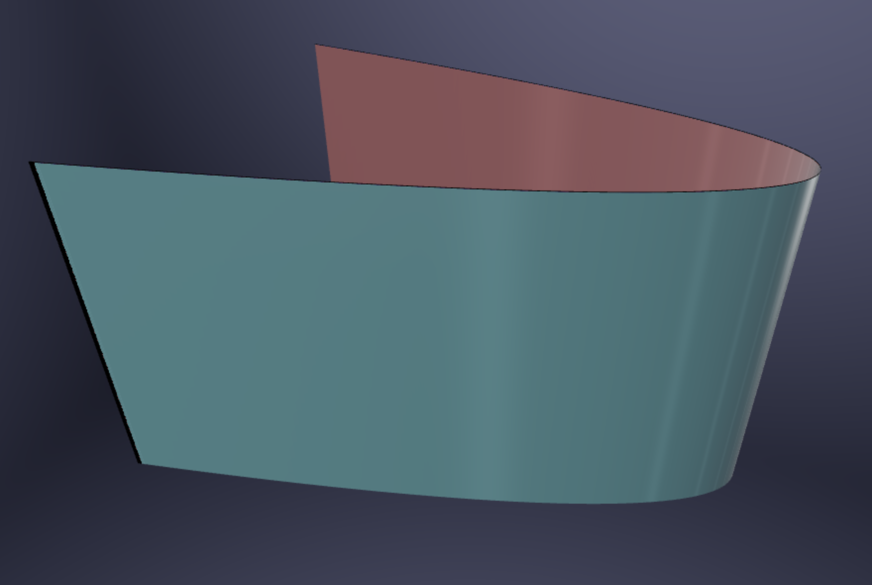
Example 4.1 (Cylinder) A cylinder is a set of points in $\RR^3$ which project orthogonally onto a circle in some plane. That is, a “stack of circles” along some axis.

The easiest examples are cylinders around coordinate axes: For example, $x^2+y^2=1$ is a circle in $\RR^2$ but is a cylinder in $\RR^3$, as the $x,y$ coordinates make a circle but the $z$ coordinate is free to be anything.

Similarly, $y^2+z^2=4$ is a circle of radius $2$ around the $x$-axis.

In general, the implicit equation of any 2-d shape can be used in 3 dimensions to describe a “stack” of those two dimensional shapes along the direction of the variable that’s missing from the formula.

Example 4.2 The equation $y=x^2$ traces out a Parabolic cylinder, that is, a stack of parabolas in the $z$-direction.

The parabolic cylinder $y=x^2$ in $\RR^3$.

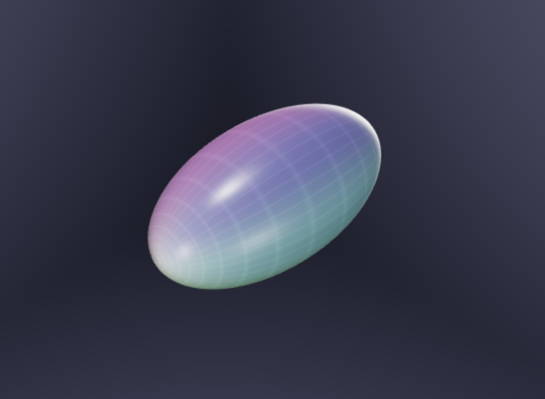
Other shapes that will be useful are ellipsoids, which are squashed spheres:

Example 4.3 (Ellipsoid) An ellipsoid is given by the implicit equation \[\frac{x^2}{a^2}+\frac{y^2}{b^2}+\frac{z^2}{c^2}=1\] This is similar to the equation of an ellipse but with one more variable.

The ellipsoid $\frac{x^2}{2}+y^2+z^2=1$ in $\RR^3$.

Example 4.4 (Paraboloid) A paraboloid is the surface $z=x^2+y^2$, or a stretched version $z=ax^2+by^2$ where $a$ and $b$ are positive. Its cross sections are circles (in the first case) and ellipses (in the second).

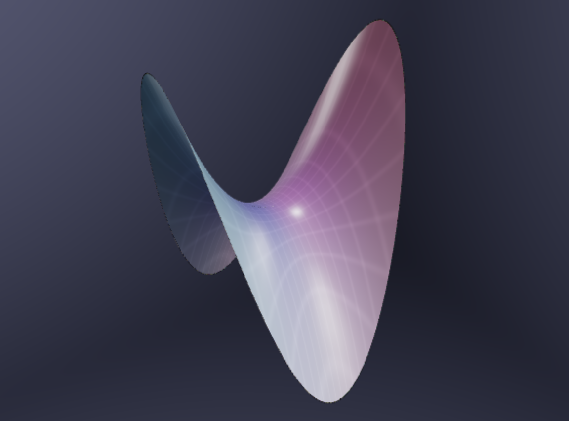
Example 4.5 (Saddle) A saddle shaped surface, or hyperbolic paraboloid is a surface of the form $z=x^2-y^2$ or a scaling of it. In this form, it has a cross section like a upwards-facing parabola along the $x$ axis, and a downwards-facing parabola along the $y$ axis.