$$ \newcommand{\RR}{\mathbb{R}} \newcommand{\QQ}{\mathbb{Q}} \newcommand{\CC}{\mathbb{C}} \newcommand{\NN}{\mathbb{N}} \newcommand{\ZZ}{\mathbb{Z}} \newcommand{\EE}{\mathbb{E}} \newcommand{\HH}{\mathbb{H}} \newcommand{\SO}{\operatorname{SO}} \newcommand{\dist}{\operatorname{dist}} \newcommand{\length}{\operatorname{length}} \newcommand{\uppersum}[1]{{\textstyle\sum^+_{#1}}} \newcommand{\lowersum}[1]{{\textstyle\sum^-_{#1}}} \newcommand{\upperint}[1]{{\textstyle\smallint^+_{#1}}} \newcommand{\lowerint}[1]{{\textstyle\smallint^-_{#1}}} \newcommand{\rsum}[1]{{\textstyle\sum_{#1}}} \newcommand{\partitions}[1]{\mathcal{P}_{#1}} \newcommand{\erf}{\operatorname{erf}} \newcommand{\ihat}{\hat{\imath}} \newcommand{\jhat}{\hat{\jmath}} \newcommand{\khat}{\hat{k}} \newcommand{\pmat}[1]{\begin{pmatrix}#1\end{pmatrix}} \newcommand{\smat}[1]{\left(\begin{smallmatrix}#1\end{smallmatrix}\right)} $$

14  Constrained Optimization

Realistic optimization problems often involve some sort of a constraint:

• What is the best product we can make, with a fixed budget?
• What is the most efficient rocket we can build of a fixed mass?
• What is the least expensive building design, given the external factors of material and labor costs?

Abstractly, all of these questions ask the following: what are the extreme values of \(f(x,y)\) given that we constrain the points \((x,y)\) by some function, \(g(x,y)=c\)? In this section, we learn a couple methods to deal with such questions.

14.1 Method I: Reduce Dimension by Substitution

The first method is just to solve the constraint for one of the variables, and substitute it into the function you wish to optimize. This forces the inputs to that function to obey the constraint - so now you can just

Example 14.1 Maximize \(z=4-2x^2-3y^2+x-y\) subject to the constraint \(x+y-2\).

This also works in higher dimensions: we can take a problem of three variables with one constraint and turn it into a problem of two variables with no constraints:

Example 14.2 Find the maximum value of \(xyz\) subject to the constraint \(x+y+z=1\).

Unfortunately, this entire method relies on being able to solve the constraint for a given variable, and substitute it in! But this is often impossible. Most relations of two variables can’t be solved for one or the other variable indpendently.

14.2 Method II: Lagrange Multipliers

What are we to do, if we cannot substitute the constraint in? It helps to back up and think geometrically here: in a two variable problem, we can draw the function \(z=f(x,y)\) as a surface in \(\RR^3\), and the constraint \(g(x,y)=c\) as a curve in the domain (the \(xy\) plane). The values of \(f(x,y)\) which satisfy the constraint

Looking for maxima along a constraint.

It’s even more helpful to draw this as a contour plot with level sets. The constraint (our hiker’s trajectory) still appears as a curve, but we can easily read off exactly where our hiker is going uphill or downhill by looking at how they are crossing contours.

Viewing a constraint problem with level sets.

Whenever the hiker is crossing a contour they are either increasing or decreasing in elevation, and so cannot be at an extremum. Indeed - extrema can only occur at locations where the hiker is not crossing a level set - that is, where their path is tangent to a level set! This is the fundamental insight

The fundamental insight of constrained optimization.

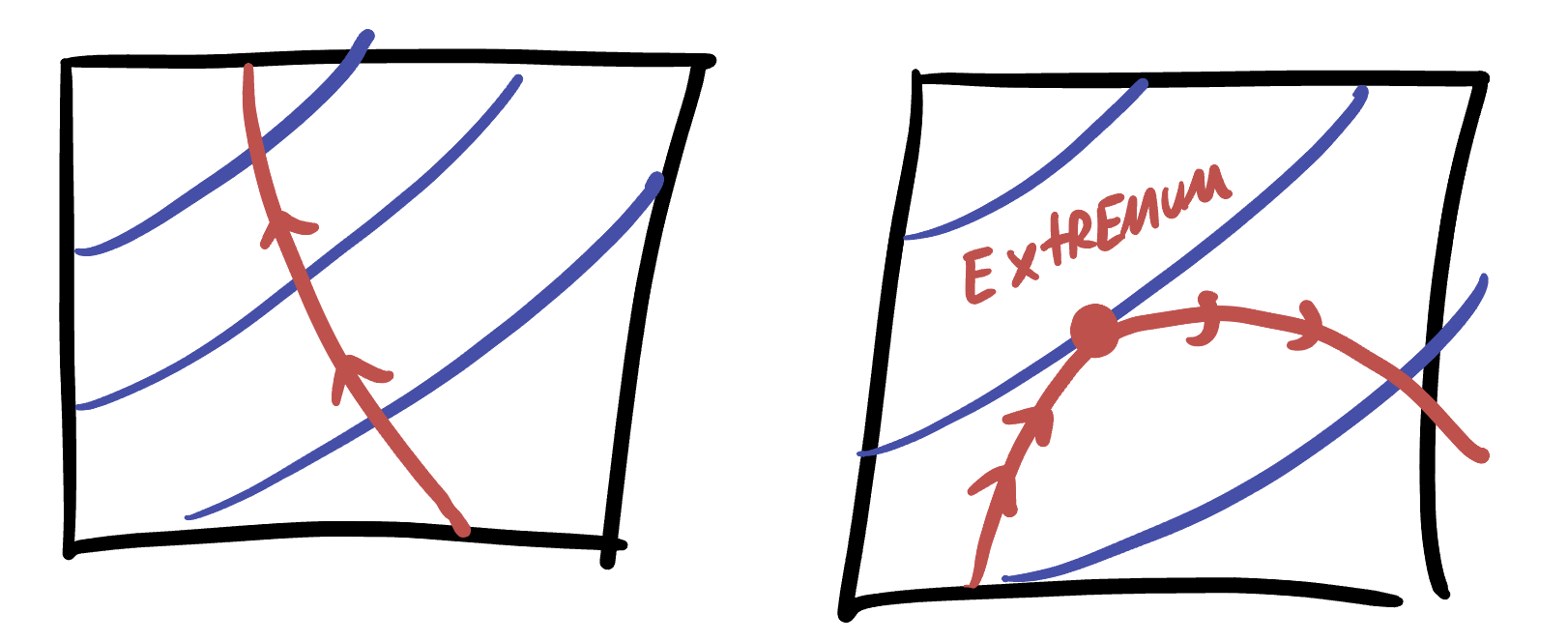
Extrema occur when the constraint is tangent to a level set.

Everything follows from this: but the work is in turning this qualitative insight into a system of equations. The first observation we can make is that the constraint itself \(g(x,y)=c\) is a level set - just of a different function. So

Extreme values of \(f\) along the constraint \(g(x,y)=c\) occur when this constraint level set is tangent to a level set of \(f\).

But this relation of is tangent to is still difficult to deal with. To help, we remember that the gradient vector is perpendicular to level sets! Thus, \(\nabla f\) and \(\nabla g\) are both perpendicular to their level sets, and thus these vectors must be parallel since the level sets are tangent.

Extreme values of \(f\) occur along \(g(x,y)=c\) whenever \(\nabla f\) is parallel to \(\nabla g\).

Now we’ve really made some progress! We just need to remember that parallel means are scalar multiples of each other and give this scalar multiple a name: it’s traditional name is the greek letter \(\lambda\)

Extreme values of \(f\) occur along \(g(x,y)=c\) when there exists a constant \(\lambda\) with \(\nabla f = \lambda \nabla g\).

This is now a fully precise, quantitative claim: it tells us that we can find the constrained extrema by solving a system of equations!

\[\left\{\begin{matrix}\nabla f(x,y,) = \lambda \nabla g(x,y)\\g(x,y)=c\end{matrix}\right\}\]

Recalling that the gradient is the vector of partial derivatives, this is just the system of equations

\[\left\{\begin{matrix} f_x(x,y)=\lambda g_x(x,y)\\ f_y(x,y)=\lambda g_y(x,y)\\ g(x,y)=c \end{matrix}\right\}\]

This has three variables and three unknowns, so generically we will be able to find some finite number of solutions! Unfortunately there is no general strategy for solving such equations, other than the “substitute one into the other and think about it” technique familiar from precalculus.

It’s illustrative to re-do the original example from the substitution section using the method of multipliers. :::{#exm-lagrange-1} Maximize \(z=4-2x^2-3y^2+x-y\) subject to the constraint \(x+y-2\). :::

Example 14.3 Maximize \(x^2+2y^2\) subject to the constraint \(x^2+y^2=1\)

Example 14.4 Find the maximum value of \(xyz\) subject to the constraint \(x+y+z=1\).

14.3 Optimization and Inequalities:

For dealing with an inequality, we need to break the problem into two cases: when the constraint is an equality, we can do the same process we have been learning above, with either Lagrange multipliers or substitution. And, inside of the constraint, we can do our more standard two dimensional optimization (finding critical points, sorting into maxes and mins), and be careful only to consider critical points that are inside the domain we care about: if the constraint is x^2+y2<1$ and you find a critical point \((3,0)\) you can ignore it, but the critical point \((1/2, 1/2)\) needs to be considered.

This will result in you having two sets of potential extrema: those occurring on the inside, and those occurring on the boundary. How do you find the absolute max (or min)? That’s easy! Just take the largest (or smallest) overall result.

Example 14.5 Maximize \(x^2+2y^2\) subject to the constraint \(x^2+y^2\leq 1\)