$$ \newcommand{\RR}{\mathbb{R}} \newcommand{\QQ}{\mathbb{Q}} \newcommand{\CC}{\mathbb{C}} \newcommand{\NN}{\mathbb{N}} \newcommand{\ZZ}{\mathbb{Z}} \newcommand{\EE}{\mathbb{E}} \newcommand{\HH}{\mathbb{H}} \newcommand{\SO}{\operatorname{SO}} \newcommand{\dist}{\operatorname{dist}} \newcommand{\length}{\operatorname{length}} \newcommand{\uppersum}[1]{{\textstyle\sum^+_{#1}}} \newcommand{\lowersum}[1]{{\textstyle\sum^-_{#1}}} \newcommand{\upperint}[1]{{\textstyle\smallint^+_{#1}}} \newcommand{\lowerint}[1]{{\textstyle\smallint^-_{#1}}} \newcommand{\rsum}[1]{{\textstyle\sum_{#1}}} \newcommand{\partitions}[1]{\mathcal{P}_{#1}} \newcommand{\erf}{\operatorname{erf}} \newcommand{\ihat}{\hat{\imath}} \newcommand{\jhat}{\hat{\jmath}} \newcommand{\khat}{\hat{k}} \newcommand{\pmat}[1]{\begin{pmatrix}#1\end{pmatrix}} \newcommand{\smat}[1]{\left(\begin{smallmatrix}#1\end{smallmatrix}\right)} $$

12 The Gradient

12.1 Directional Derivatives

We have seen that $\partial_x f$ and $\partial_y f$ measure the slope of a multivariate function in the $x$ and $y$ directions, respectively. But what is its rate of change in the direction of an arbitrary unit vector $u$?

Definition 12.1 (Directional Derivative) The derivative of $f$ in the direction of a unit vector $u$ is denoted $D_uf$ and is defined by the limit

\[\lim_{h\to 0}\frac{f(p+\epsilon u)-f(p)}{\epsilon}\]

Computing this seems difficult. But we can use the Fundamental Strategy of Calculus to save the day! We know that the slope in the direction $u$ must lie on the tangent plane, which we have already parameterized in terms of the $x$ and $y$ partials:

\[\mathrm{Plane}(s,t)=\pmat{x \\ y\\ f(x,y)}+ s\pmat{1\\ 0\\ \partial_x f}+t \pmat{0\\1\\ \partial_yf}\]

We can plug $u=\langle a,b\rangle$ in here and take a look at the $z$ coordinate to read off the change in $z$. \[ z =f(x,y)+a \partial_x f + b\partial_y f\]

So the change in $z$ is just the quantity $a\partial_x f+b\partial_y f$. Alternatively, we can use the differential we derived from this linear approximation \[dz = f_x dx+f_y dy\] To see if $dx=a$ and $dy=b$ that $dz=af_x+bf_y$. It’s just a linear combination of the two basic slopes we already know!

Theorem 12.1 (Directional Derivative) If $u=\langle a,b\rangle$ is a unit vector, then \[D_uf(x,y)=af_x(x,y)+bf_y(x,y)\]

All of this carries over to three or higher dimensions: if $u=\langle a,b,c\rangle$ and $f(x,y,z)$ is a three variable function then

\[D_u f = af_x+bf_y+cf_z\]

12.2 The Gradient

Because the collection of partial derivatives $\langle f_x,f_y\rangle$ will show up so often it will be useful to give this a name: the gradient.

Definition 12.2 (The Gradient) The gradient of a function $f(x,y)$ is \[\nabla f=\langle f_x,f_y\rangle\] The gradient of $f(x,y,z)$ is the 3-dimensional vector \[\nabla f = \langle f_x,f_y,f_z\rangle\]

Definition 12.3 (Nabla) The symbol $\nabla$ is called nabla or del, and is a shorthand for the vector of partial derivative operators: \[\nabla = \langle \partial_x,\partial_y,\partial_z\rangle\]

This notation is convenient here as

\[\begin{align*} \nabla f &= \langle \partial_x, \partial y\rangle f\\ &=\langle \partial_x f,\partial_y f\rangle\\ &=\langle f_x,f_y\rangle \end{align*}\]

But it will also be convenient later in the course, for defining other types of derivatives. A first benefit here is it can take our formula for the directional derivative and make it much simpler to remember!

Theorem 12.2 (Directional Derivatives and the Gradient) \[D_u f(x,y)=\nabla f\cdot \hat{u}\]

12.3 Geometry of the Gradient

Since we know the interpretation of dot products in terms of angles, we can use the directional derivative formula above to help us understand the direction the gradient points in.

If a vector $u$ makes angle $\theta$ with the gradient, we see the directional derivative in direction $u$ is given by

This actually tells us alot!

Theorem 12.3

The gradient points in the direction of maximal directional derivative.
Its magnitude is the directional derivative in that direction
In the orthogonal direction to the gradient, the directional derivative is zero: the function is not changing!

Open Fullscreen

The last of these facts is so useful on its own, that it gets it’s own theorem box:

Theorem 12.4 The gradient vector is orthogonal to the level sets of a function, and points in the direction of increase.

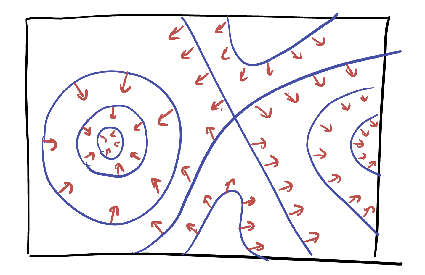
The gradient is orthogonal to level sets.

This is very helpful for understanding a function from its gradient, as it lets us convert between level set understanding and gradient understandings!

The gradient points in the direction of steepest ascent.

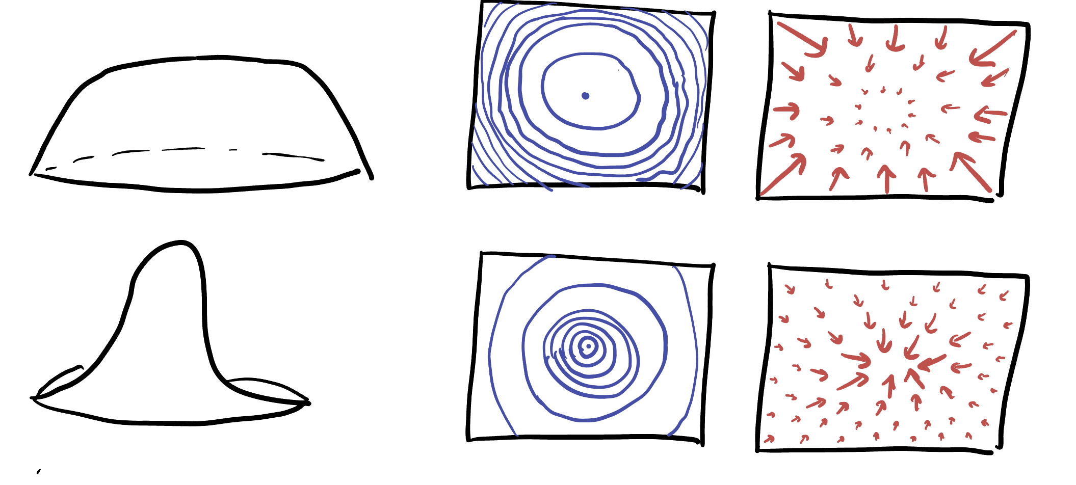
12.3.0.1 The Gradient and Level Sets

When level sets are close to each other, that means the function is steeply increasing or decreasing, so the gradient is long. When level sets are far apart, that means the function is only slowly changing, so the gradient is short. Thus, there’s an inverse relationship between the length of the gradient and the density of level sets.

The length of the gradient is inversely proportional to the density of contour lines.

12.3.1 Tangent Planes to Level Sets

Because the gradient is a normal vector to level sets we can use the gradient to derive the equation for a tangent plane to a surface! We previously wrote it down of for functions,

\[f_x(a,b,c)(x-a)+f_y(a,b,c)(y-b)+f_z(a,b,c)(z-c)=0\]

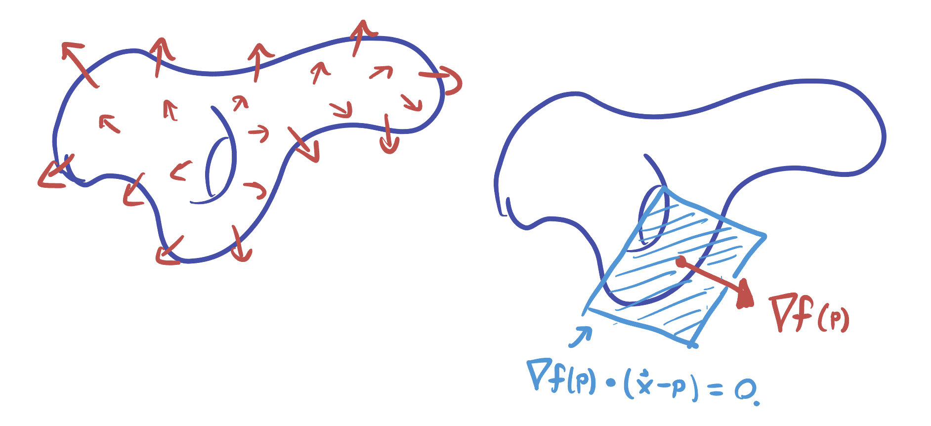
But this was just in analogy with the tangent line case. Now, we wish to derive it from our original description of planes, in terms of their normal vectors: if $p$ is a point on the plane and $n$ is a normal vector to the plane, the equation

\[n\cdot ((x,y,z)-p)=0\]

Describes the plane because it says $(x,y,z)$ lies in the plane so long as the vector connecting it to $p$ is orthogonal to $n$. Now that we know the gradient \[\nabla f(a,b,c)=\langle f_x(a,b,c), f_y(a,b,c),f_z(a,b,c)\rangle\]

is the normal vector to our plane, we can directly write down the equation for the normal at $(a,b,c)$:

\[\nabla f(a,b,c)\cdot ((x,y,z)-(a,b,c))=0\]

and, after computing the dot product we can see it’s the same equation we already know!

The gradient is normal to level sets, even in 3D. This makes it easy to use the gradient to find the tangent plane to a level set.

But knowing the normal vector also allows us to compute other geometric quantities of interest: such as the normal line: the parametric line which intersects a level set orthogonally.

The normal line to a level set in three variables.

This is also immediate: as if we know a point $p$ and a direction vector $v$, the associated line is $\ell(t)=p+tv$. So here, the point is $(a,b,c)$ and the normal vector is $\nabla f(a,b,c)$ so the normal line is

\[\ell(t)=(a,b,c)+ t \nabla f(a,b,c) \]

Example 12.1 Compute the tangent plane and the normal line to $x=y^2+z^2+1$ at $(3,1,-1)$.

First, we re-arrange so that the surface equation is written as a level set: $x-y^2-z^2=1$ with all the variables on one side. Now we can compute the gradient:

\[\nabla f =\langle 1,-2y,-2z\rangle\hspace{1cm}\nabla f(3,1,-1)=\langle 1,-2,2\rangle\]

This vector and the original point $(3,1,-1)$ immediately determine the plane and line:

\[\langle 1,-2,2\rangle\cdot \langle x-3,y-1,z+1\rangle=0\] \[x-2y+2z=-1\]

\[\ell(t)=(3,1,-1)+t\langle 1,-2,2\rangle =(3+t,1-2t,-1+2t)\]