6 Calculus
(Relevant Section of the Textbook: 13.2 Derivatives and Integrals of Vector Functions)
A parametric curve is made of \(n\) component functions, which are familiar functions \(\RR\to\RR\) from single variable calculus. Thus, the calculus of curves is simply doing the calculus of single variable functions \(n\) times!
6.1 Limits
Taking limits of a parametric curve is just taking the limit of each component function.
Definition 6.1 (Limits of Parametric Curves) If \(\vec{r}(t)=(x(t),y(t),z(t))\) is a parametric curve, then limits are computed componentwise: \[\lim_{t\to a}r(t)=\left(\lim_{t\to a}x(t),\lim_{t\to a}y(t),\lim_{t\to a}z(t)\right)\]
Example 6.1 (Limits of Parametric Curves) Let \(\vec{r}(t)\) be the following parametric curve \[\vec{r}(t)=\left\langle \frac{1}{t+1},\frac{\sin(t)}{t}, \frac{3t+t^2}{t}\right\rangle\] Compute the limit \(\lim_{t\to 0}\vec{r}(t)\).
Computing the limit componentwise we see we just need to evaluate three limits:
\[\lim_{t\to 0}\frac{1}{t+1}\] \[\lim_{t\to 0}\frac{\sin(t)}{t}\] \[\lim_{t\to 0}\frac{3t+t^2}{t}\]
The first of these is continuous at zero so we can just plug in. THe second need L’Hospital’s rule, and the third needs us to cancel a \(t\) from the numerator and denominator before plugging in, to get
\[\lim_{t\to 0}\vec{r}(t)=\langle 1,1,3\rangle\]
6.2 Differentiation
Recall the single variable definition of the derivative:
\[f^\prime(t)=\lim_{h\to 0}\frac{f(t+h)-f(t)}{h}\] The same definition works for parametric curves:
Definition 6.2 (Differentiating Curves) The derivative of a parametric curve \(\vec{r}(t)\) at a point \(t\) is given by the following limit:
\[\lim_{h\to 0}\frac{\vec{r}(t+h)-\vec{r}(t)}{h}\]
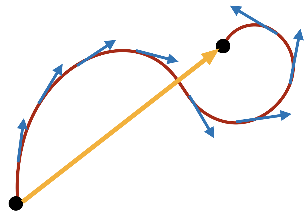
The numerator here is a vector, which gets infinitesimally small as \(h\to 0\), connecting two closer and closer together points of the curve. We then rescale this vector with scalar multiplication, dividng by \(h\) to keep the vector’s length from collapsing. In the limit, this converges to a vector \(\vec{r}^\prime(t)\) which is tangent to the curve.
However, we don’t need to calculate the derivative using this limit statement every time! We can use the fact that limits distribute over the components of the function to prove that we can also take the derivative one component at a time.
Theorem 6.1 (Differentiating Curves Componentwise) If \(\vec{r}(t)=(x(t),y(t),z(t))\) is a parametric curve, then \[\vec{r}^\prime(t)=\langle x^\prime(t),y^\prime(t),z^\prime(t)\rangle\]
Because of this, its straightforward to show that differenatiation of vector functions obeys the familiar laws of single variable calculus: you can break it up over sums, and pull out scalars. But now there are three types of products (do we multiply the vector function by a scalar function, or dot or cross product it with another vector?)
Theorem 6.2 (Differentiation Product Laws) \[\left(f(t)\vec{r}(t)\right)^\prime= f^\prime(t)\vec{r}(t)+f(t)\vec{r}^\prime(t)\] \[\left(\vec{c}(t)\cdot\vec{r}(t)\right)^\prime = \vec{c}^\prime(t)\cdot \vec{r}(t)+\vec{c}(t)\cdot \vec{r}^\prime(t)\] \[\left(\vec{c}(t)\times\vec{r}(t)\right)^\prime = \vec{c}^\prime(t)\times \vec{r}(t)+\vec{c}(t)\times \vec{r}^\prime(t)\]
There is also a chain rule: we can’t compose a vector function inside another vector function, but we can plug a scalar function in as the parameter in a curve!
Theorem 6.3 (The chain rule) \[\left(\vec{r}(f(t))\right)^\prime=\vec{r}^\prime(f(t))f^\prime(t)\]
You probably notice a similarity to the single variable calculus versions in all of these: they’re as close as possible, except now being about vector functions! But these simple looking rules actually provide us a new powerful set of tools, they tell us about the rate of change at the same time as dot and cross products - which we know can measure areas and angles!
As one quick example, we’ll prove a very useful fact about curves defined by vectors of constant length.
Theorem 6.4 (Curves on the Sphere) If a curve \(\vec{r}(t)\) never changes in length, so \(\|\vec{r}(t)\|=k\) for all time, then \(\vec{r}^\prime\) is orthogonal to \(r\).
Proof. Since the magnitude of a vector can be calculated from its dot product, we see that \[\vec{r}\cdot \vec{r}=k^2\] Taking the derivative of this with the product rule, we find \[\vec{r}^\prime \cdot \vec{r}+\vec{r}\cdot\vec{r}^\prime = 0\]
The dot product is commutative (order doesnt matter) so we can re-arrange the left hand side:
\[2\vec{r}\cdot \vec{r}^\prime =0\]
But dividng by two - this says that the dot product of \(\vec{r}\) and \(\vec{r}^\prime\) is zero! So these two vectors are orthogonal.
6.3 Integration
The story of vector valued integration is similarly straightforward. Recall the definition of integration via Riemann sum:
\[\int_a^b f(x)dx=\lim_{N\to\infty}\sum_{i=1}^N f(x_i)\Delta x\]
We can apply the same definition to vector valued functions, as its composed of just the operations of addition and scalar multiplication!
Definition 6.3 (Integrating Curves) If \(\vec{r}\) is a parametric curve, its vector valued integral on the interval \([a,b]\) is defined by the following Riemann sum:
\[\int_a^b\vec{r}(t)dt = \lim_{N\to\infty }\sum_{i=1}^N \vec{r}(t_i)\Delta t\]
But wait! Both scalar multiplication and addition are things we can do componentwise for a vector. So we can break this big Riemann sum up into a standard riemann sum in each component. Taking the limit, this tells us we can integrate vector functions componentwise.
Theorem 6.5 (Integrating Curves Componentwise) If \(\vec{r}(t)=\langle x(t),y(t),z(t)\rangle\), the vector valued integral of \(\vec{r}\) on \([a,b]\) is given by \[\int_a^b \vec{r}(t)dt = \left\langle \int_a^b x(t)dt, \int_a^b y(t)dt, \int_a^b z(t)dt\right\rangle\]
We will only find limited use of this in our class, as there are other types of integrals along curves that will prove more important. Nonetheless this does show up in many applications of multivariable calculus to engineering and physics, where one may wish to recover position from velocity, or velocity from acceleration.
Example 6.2 (Displacement from Veloicty) If \(\vec{v}(t)\) is a parametric curve giving the velocity of a particle at time \(t\), then \(\int_a^b \vec{v}(t)dt\) is teh displacement vector for its net travel between \(t=a\) and \(t=b\).
The same is true for acceleration: all of our phones have a sensor inside called a three axis accelerometer. These measure the acceleration as a function of time
\[\vec{a}(t)=\langle a_x(t),a_y(t),a_z(t)\rangle\]
But this is not what software running on the phone wants or needs: it cares about your position in space! (Say, if you’re using your phone in augmented reality). To get this, it integrates the acceleration to get velocity, and then integrates again the veloctity to get position! P For any engineers in the class - if you have accelerometers in the Hive: this could be a fun project to code up! Write a small python program to numerically integrate (ie compute a Riemann sum) from the output data of an accelerometer, and track your hand’s position as you move it around.
6.4 Videos
Calculus Blue series on calculus of curves:
Here are some videos practicing the concepts that we have done examples of in lecture. First, limits of vector functions.
Next, derivatives of vector functions.
And the proofs of the differentiation laws for the dot product and cross product:
Also, integrating vector functions.