10 Linearization & Approximation
10.1 The Fundamental Strategy of Calculus
Take a complicated function, zoom in, replace it with something linear. Thus we are looking to replace graphs by planes. To start, look back on the tangent line formula from single variable calculus:
\[y=y_0+f^\prime(x_0)(x-x_0)\]
Our extension to multiple dimensions is just….to add more variables! We need to adjust \(z\) not just for changes in \(x\) any more, but also for changes in any input.
Theorem 10.1 (Tangent Plane) \[z=z_0+f_x(x_0,y_0)(x-x_0)+f_y(x_0,y_0)(y-y_0)\]
Because the tangent plane is the best linear approximation to a function at a point, it is often called the Linearization
Same formula works in higher dimensions, by just adding more terms. Since this gives us an implicit plane, we can re-arrange this to the “standard form” and find the normal vector to the graph
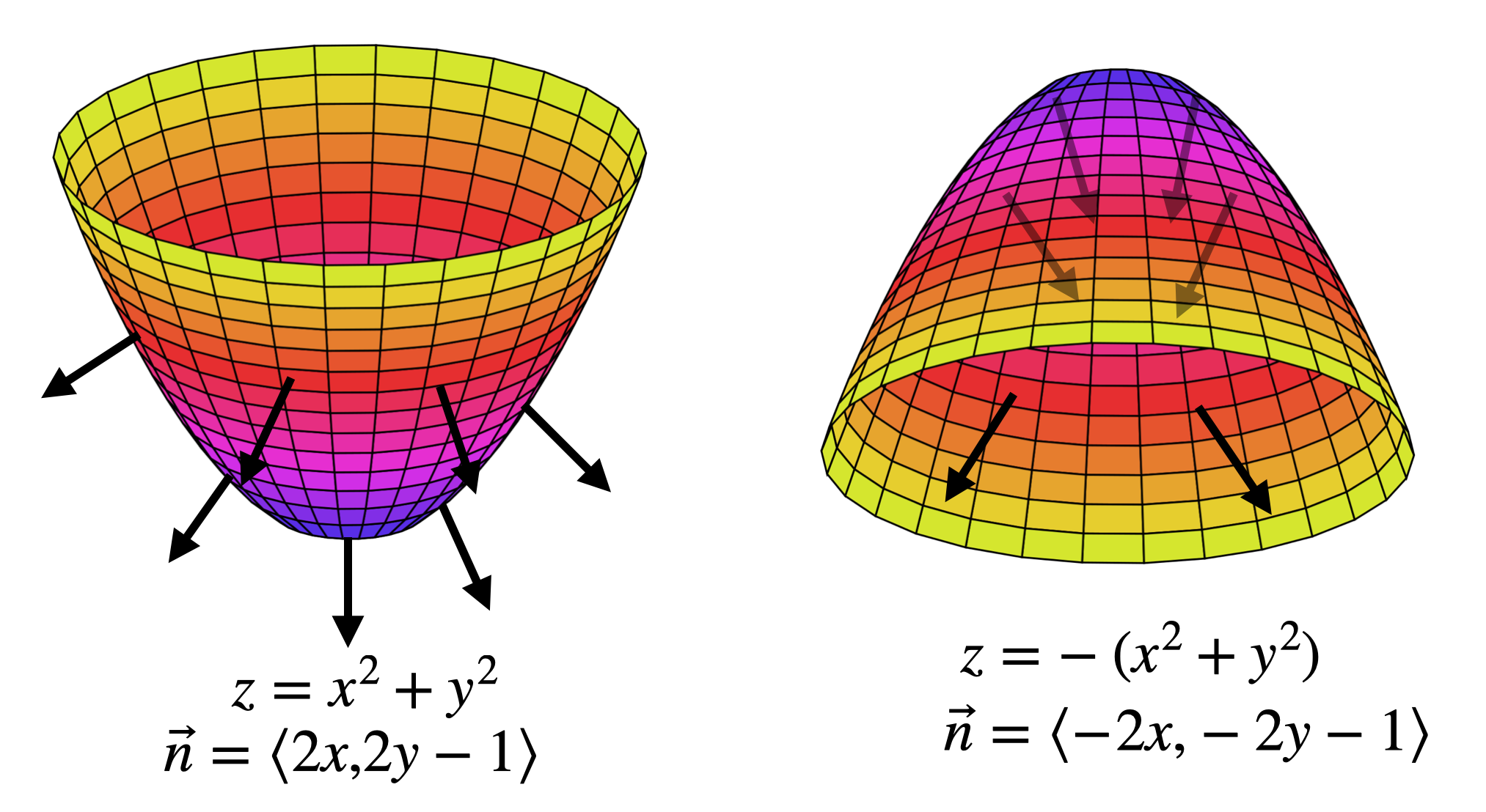
Theorem 10.2 (Normal Vector to a Graph) At the point \((x_0,y_0)\) the plane \[f_x(x_0,y_0)(x-x_0)+f_y(x_0,y_0)(y-y_0)-z=-z_0\] is tangent to the graph of \(f\). Thus, the normal vector is the coefficient vector \[n=\langle f_x(x_0,y_0),f_y(x_0,y_0),-1\rangle\]
Note that any scalar multiple of this vector is also a normal vector to the graph - this just provides one such vector. And, since the \(z\) is downwards, this is the downwards pointing normal vector.
Depending on the application, sometimes we want the upward facing normal: that’s what you’d get by multiplying this by \(-1\) so that the last coordinate is a 1:
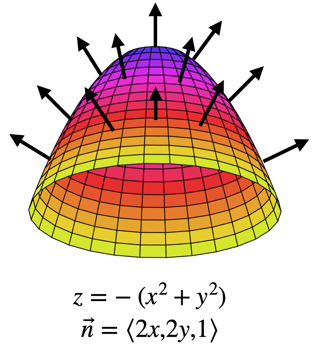
We will use normal vectors to surfaces a lot in the last portion of this course, on Vector Analysis. Here we will often need to be careful, and thinking about whether we want the normal that is pointed up or down in a given application.
Example 10.1 Find the tangent plane to \(z=x^2+2y^2\) above the point \((x,y)=(2,3)\).
The differentiability of a function in multiple variables is defined in terms of the existence of a tangent plane: we say that a function \(f(x,y)\) is differentiable at a point \(p\) if there exists some tangent plane that well-approximates it at that point. Functions we will see are mostly differentiable, but warning there are functions that are not. Luckily, there’s an easy way to check using partial derivatives:
Theorem 10.3 (Multivariate Differentiability) A multivariate function is differentiable at a point, if and only if all of its partial derivatives exist and are continuous at that point.
10.2 Differentials
The Fundamental Strategy of calculus is to take a complicated nonlinear object (like a function that you encounter in some real-world problem) and zoom in until it looks linear. Here, this zooming in process is realized by finding the tangent plane. Close to the point \((x_0,y_0)\) the graph of the function \(z=f(x,y)\) looks like \[L(x,y)=z_0+f_x(x_0,y_0)(x-x_0)+f_y(x_0,y_0)(y-y_0)\]
Where \(z_0=f(x_0,y_0)\). This is just rehashing our definition of the tangent plane of course: but one use for it is to be able to approximate the value of \(f(x,y)\) if you know the value of \(f\) at a nearby point \((x_0,y_0)\) and also its partial derivatives there.
Example 10.2 Find approximate value value of \(x^2+3xy-y^2\) at the point \((2.05,2.96)\).
Using linearization to estimate changes in a value: fundamental to physics and engineering. In 1-dimension, we define a variable called \(dx\) that we think of as measuring small changes in the input variable, and \(dy=y-y_0\) which measures small changes in the output. These are related by
\[dy=f^\prime(x)dx\]
So, any change in the input is multiplied by the derivative to give a change in the output. We can do a similar thing in more variables. For a function \(f(x,y)\), we have the tangent plane above \[z=z_0+f_x(x_0,y_0)(x-x_0)+f_y(x_0,y_0)(y-y_0)\]
Subtracting \(z_0\) and setting \(dz=z-z_0\), and similarly for \(dx,dy\) we can rewrite this as below:
Definition 10.1 (Differentials) \[dz=f_x(x,y)dx+f_y(x,y)dy\]
This allows us to easily estimate how much \(z\) could change if we know how much \(x\) and \(y\) can change. This is of fundamental importance in error analysis, the foundation of all experimental science’s ability to compare with theoretical predictions.
Example 10.3 The volume of a cone is given by \(V=\pi r^2 h/3\). We have a cone which we measure the height to be 10cm and the radius to be 25cm, but our measuring device can have an error up to 1mm or \(0.1cm\). What is the estimated maximal error in volume our measurement could have?
This measurement can also be interpreted geometrically: this is the approximate volume of a thin-shelled cone of thickness \(1mm\) with radius 25cm and height 10cm.
Example 10.4 The dimensions of a rectangular box are measured to be 75cm, 60cm and 40cm. Each measurement is correct to within \(0.05cm\). What is the maximal error in volume measurement we might expect?
10.3 Quadratic Approximations
We’ve already gotten a ton of use out of linear approximations to a multivariable function. But we can learn even more by proceeding to higher derivatives. Here we study the quadratic approximation that includes all the first and second derivative information. Like in the linear case, the best way to get started is to recall what happens in one variable for the second order term in a taylor series:
\[f(x)\cong f(a)+f^\prime(a)(x-a)+\frac{1}{2}f^{\prime\prime}(a)(x-a)^2\]
The move to multiple variables for the linearization required us just tacking on analogous terms for all additional variables. Happily the same holds true here!
Definition 10.2 (Quadratic Approximation) If \(f(x,y)\) is a differentiable function of two variables, its quadratic approximation at a point \((a,b)\) is
\[\begin{align} f(x,y) & \approx f(a,b)+f_x(a,b)(x-a)+f_y(a,b)(y-b)+\\ &+ \frac{1}{2}\left(f_{xx}(a,b)(x-a)^2+f_{xy}(a,b)(x-a)(y-b)+f_{yx}(a,b)(y-a)(x-b)+f_{yy}(a,b)(y-b)^2\right) \end{align}\]
Because we know the order in which we take partials doesn’t matter, \(f_{xy}=f_{yx}\) and so this simplifies to
\[\begin{align} f(x,y) & \approx f(a,b)+f_x(a,b)(x-a)+f_y(a,b)(y-b)+\\ &+ \frac{1}{2}\left(f_{xx}(a,b)(x-a)^2+2f_{xy}(a,b)(x-a)(y-b)+f_{yy}(a,b)(y-b)^2\right) \end{align}\]
If you have taken Linear Algebra (or have seen Matrix Multiplication before elsewhere) there is a nice way to remember this formula for \(\vec{x}=(x,y)\) and \(\vec{p}=(a,b)\), writing it out in terms of row vectors, column vectors and matrices, where \(\nabla f\) is the gradient (vector of first derivatives) and \(Hf\) is the Hessian (matrix of second derivatives)
\[f(x,y)\approx f(p)+\nabla f(p)\cdot(\vec{x}-\vec{p}) + \frac{1}{2}(\vec{x}-\vec{p})\cdot Hf(p)(\vec{x}-\vec{p})\]
This formula looks intimidating in any of these forms when written out completely. But its actually super easy to remember!
- Start with the value \(f(a,b)\) at the point we know
- Add in first derivatives \(f_x(a,b)\) and \(f_y(a,b)\) multiplied by how far we’ve moved in that direction.
- Add in \(\frac{1}{2}\) each second derivative, multiplied by the differences \((x-a)(x-a)\), or \((x-a)(y-b)\) or \((y-b)(y-b)\) depending on which second derivatives were taken.
10.3.1 The Geometry of Quadratic Approximations
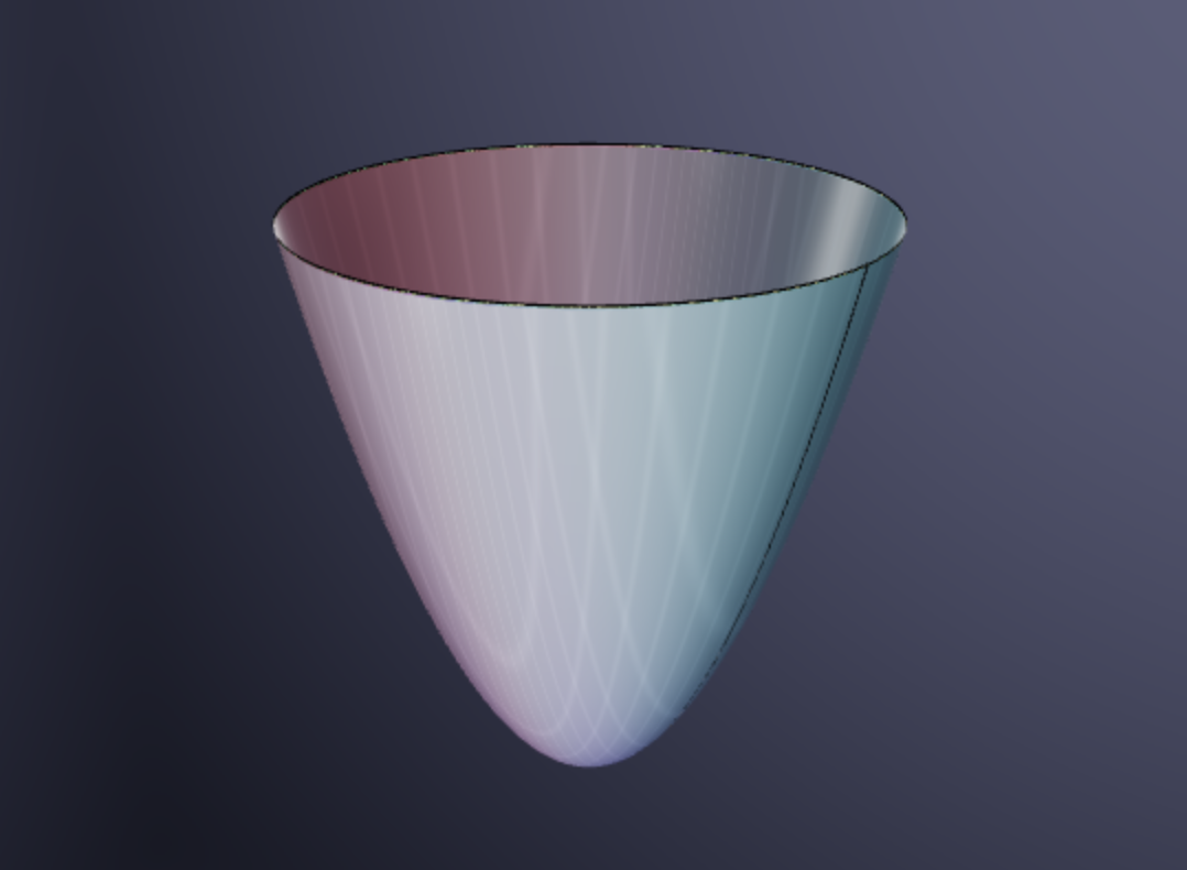
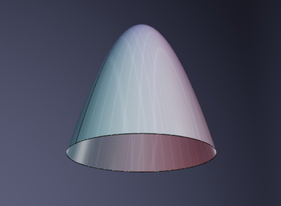
Once we have a quadratic approximation to a surface we have an even better understanding of what it looks like near a point. Of course, that requires that we know what quadratic surfaces look like - and hence why we spent time on those earlier this semester! Generic quadratic surfaces come in three types: hills, bowls and saddles
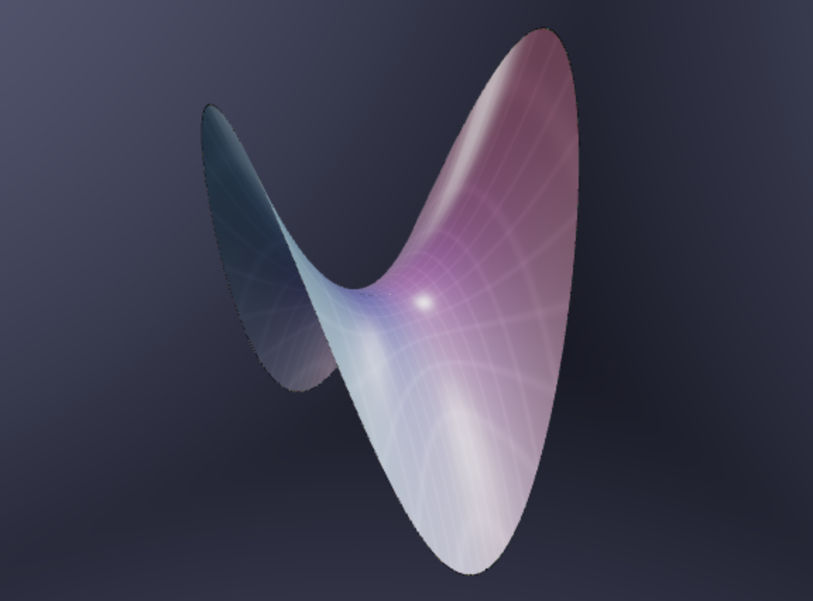
So computing the quadratic approximation to a function tells us if near that point, a portion of the surface is best approximated by a hill bowl or saddle. We can tell which by computing the quadratic approximation and taking some slices: if the slices are parabolas both opening in the same direction its either a hill or bowl, but if they open in opposite directions its a saddle.
Find a quadratic approximation to \(e^{x}y^2\) at \((1,2)\). Is this approximation a hill, bowl or saddle?
Note that just because a hill is the best approximation near a point does not mean we are at a maximum - we could just be on the side of the hill! But these tools do turn out to be extremely useful for finding maxes and mins: these can occur when the first derivatives are zero. The whole next section of the course notes is devoted to some examples of using the quadratic approximation to do exactly this.
To get a better sense of what’s going on, here’s a program that draws the quadratic approximation automatically for you.
PROGRAM
Examples of finding quadratic approximations to a function.