14 Double Integrals
We now begin a new chapter - after studying in detail various means of studying change via multivariate differentiation, we will switch to study accumulation via multivariate integration. As Calculus I and II focused on defining the integral of a single variable over a 1-dimensional region (the closed interval \([a,b]\)), we will continue in Calculus III to define the integral of multivariate functions over two and three dimensional regions.
14.1 Riemann Sums and Iterated Integrals
In one dimension, an integral measures the area under a graph by breaking in into slices, and adding up approximate areas of each slice, via a Riemann sum, before taking a limit. We will begin with a similar process here, we define the double integral of a function \(f(x,y)\) over a region \(R\) in the plane by a two dimensional Riemann sum.
This two dimensional Riemann sum works by breaking the region \(R\) into small rectangular regions which we will denote \(\Delta A\), choosing a point \((x_i, y_j)\) in each such region, and then summing \[\sum_{i=1}^N\sum_{j=1}^N f(x_i,y_j)\Delta A\]
As the number of regions goes to infinty, and the size of each rectangle \(\Delta A\) goes to zero, this becomes an integral, with \(\Sigma\) becoming \(\int\) and \(\Delta\) becoming \(d\):
\[\iint_R f(x,y)dA\]
This measures the volume under the graph of \(f\) above the region \(R\), instead of the area under a curve. But how do we evaluate this thing? We can either add up the volume of each row with constant \(x\) first, to get a function of \(y\), and then add these up, or the opposite: first add up in rows of \(y\) to get a function of \(x\), then add these up. Either way, we add up all the little volumes, and this gives the total volume under the surface.
You can see this in the animation below: where one of the side bar graphs gives the result of summing along rows first, the other columns, and these two side graphs have the same total area under their curves.
14.2 Rectangular Domains
Let \(R\) be the region \(a\leq x\leq b\) and \(c\leq y \leq d\). Say we want to compute the integral \(\iint_R f(x,y)dA\). By the observation above (Fubini’s theorem) we can compute this by integrating all the \(x\)’s first then integrating \(y\), or vice versa:
\[\iint_R f(x,y)dA = \int_a^b\left(\int_c^d f(x,y)dy\right)dx=\int_c^d\left(\int_a^b f(x,y)dx\right)dy\]
This is a massive simplification: it means that we can compute two dimensional integrals by just doing two one dimensional integrals, one after the other!
Example 14.1 Evaluate \(\iint_R x^2y\,dA\) for \(R=[1,2]\times[3,4]\)
Example 14.2 Evaluate \(\iint_R x(3-y^2)\,dA\) for \(R=[0,2]\times[1,2]\)
Oftentimes, the order one performs the integrals in does not matter - both are equally straightforward. But this is not always the case!
Example 14.3 Integrate \(y\sin(xy)\) over the region \(R=\{0\leq x\leq 1, 0\leq y\leq \pi\}\).
Try both orders, see which is easier!
Sometimes, when the function you are integrating is a product of a function of \(x\) and a separate function of \(y\), things can simplify even further! If \(f(x,y)=g(x)h(y)\) then we may write
\[\iint_R =\int_a^b\int_c^d g(x)h(y)dydx = \left(\int_a^b g(x)dx\right)\left(\int_c^d h(y)dy\right)\]
We get this by realizing that \(g(x)\) is a constant with respect to the \(y\) integral so we can pull it out: but then once we have done the \(y\) integral the result is a constant, so we can pull it out of the \(x\) integral!
Example 14.4 Compute
\[\iint_R e^x\sin(y)dA\] On the region \(R=[0,\pi/2]\times[0,\pi/2]\).
This is essentially all there is to the theory of multiple integrals when the domain is a box (where all variables are bounded by constants). Indeed, we will shortly meet triple integrals and see that everything remains precisely the same!
\[\int_R g(x,y,z)dV = \int_a^b \left(\int_c^d\left( \int_e^f g(x,y,z)dz\right)dy\right)dx\]
However, before going there we will continue on and look at more general double integrals: what happens when the region \(R\) is not a box?
14.3 Variable Boundaries
In one variable calculus, the only sort of region over which you could perform an integral is a single interval. But in two variables, the regions of the plane over which you could wish to integrate are much more varied!

We have learned how to deal with rectangular regions by slicing - and this same technique will serve us well in many other cases. To start, we won’t focus on completely general regions, but rather on regions where the top and bottom are bounded by functions of \(x\):

Here, if we slice with respect to \(y\) first, our vertical slices will each be of a different length - but they will still always be intervals (the top and bottom are functions meaning they pass the vertical line test - so each intersects the vertical strip exactly once).
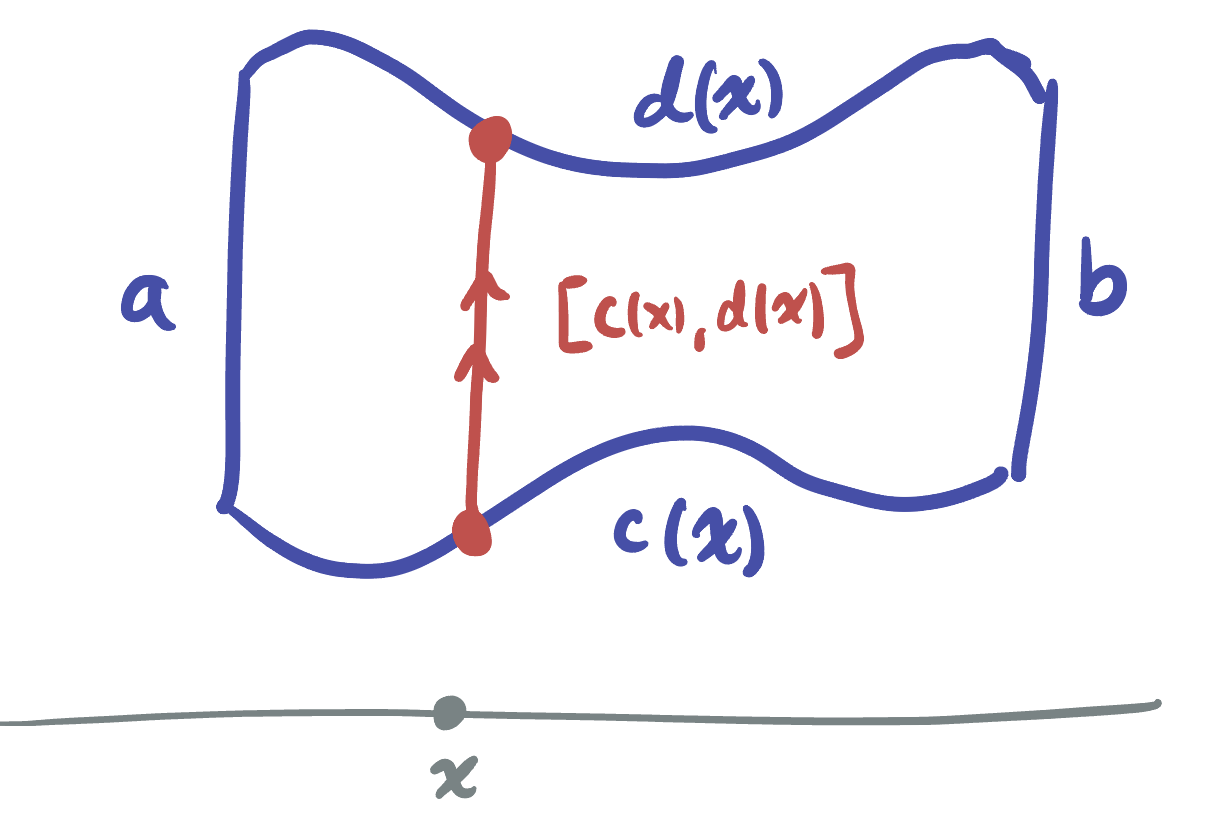
At the fixed value \(x\), what is the interval we are integrating over? Well, it runs from the bottom function \(a(x)\) to the top function \(b(x)\), and so the integral along this slice is
\[\int_{c(x)}^{d(x)}f(x,y)dy\]
Then all that remains is to integrate this along the \(y\) direction:
\[\iint_R f(x,y)dA =\int_a^b\int_{c(x)}^{d(x)}f(x,y)dydx\]
Exercise 14.1 Find the integral of \(x+2y\) over the region \(R\) \[R=\{(x,y)\mid 0<x<2\,\,\,\, x^2-2<y<x\}\]
Sometimes the \(x\) bounds don’t even need to be given explicitly-they are just the region between where the curves intersect:
Exercise 14.2 Find the volume above the \(xy\) plane under the graph of \(z=x^2+y^2\), within the region \(R\) bounded by \(y=2x\) and \(y=x^2\).
There’s nothing special about slicing with respect to the \(x\) direction, we can also do integrals by slicing with respect to fixed \(y\), and integrating \(dx\) first. Indeed, the above example can be redone this way no problem!
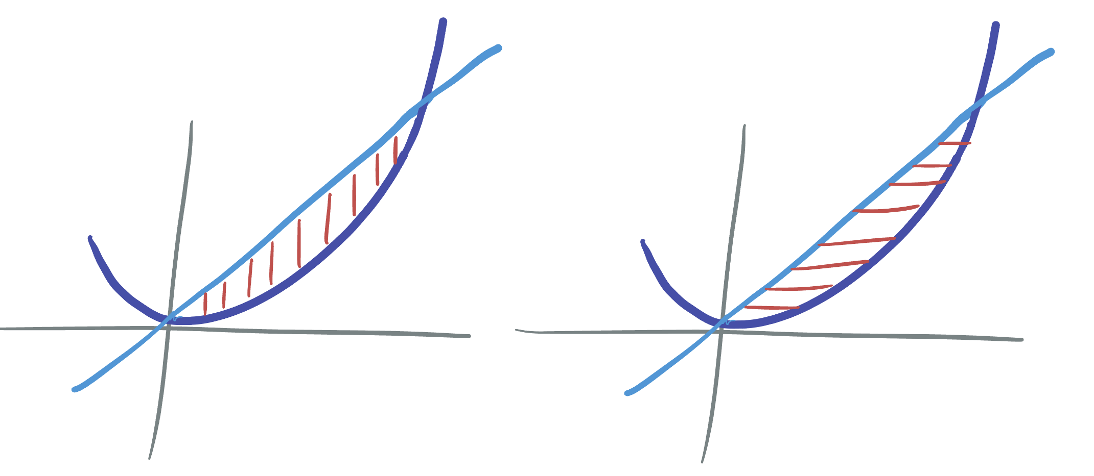
Exercise 14.3 Find the volume above the \(xy\) plane under the graph of \(z=x^2+y^2\), within the region \(R\) bounded by \(y=2x\) and \(y=x^2\), this time first slicing horizontally, with constant \(y\).
However, not every example is just as easy both ways. For example the following integral is easy to write down sliced with respect to \(y\), but harder when sliced first with constant \(x\):
Exercise 14.4 Integrate \(x+y\) on the region \(R\) determined by \[R=\{(x,y)\mid -2<y<2\,\,\,\, y^2-1<x<3\}\]
14.3.1 Changing the Order of Integration
To do the last integral instead with respect to slices of constant \(x\) (so, slices in the \(y\) direction) we would need to solve for the \(y\) bounds as a function of \(x\),
Exercise 14.5 Set up the integral of \(x+y\) on the region \[R=\{(x,y)\mid -2<y<2\,\,\,\, y^2-1<x<3\}\] Where slicing is first done at constant \(x\)s.
One of the most important things about setting up a double integral correctly is thinking through which order of integration will be more useful, and why. Sometimes, one way of slicing will lead to an impossible integral, but the other way will be easy!
Example 14.5 Compute the integral
\[\int_0^1\int_x^1 \sin(y^2)dydx\] by switching the order of integration first.
14.4 Combining Integrals
Just like there is a subdivision rule for one dimensional integrals, \[\int_a^b fdx=\int_a^c fdx+\int_c^b fdx\] There is a similar rule for double integrals: if you break the domain into two regions, the double integral over the whole thing is the sum of the double integrals over each. In symbols: if \(R=R_1\cup R_2\), then
\[\iint_R fdA = \iint_{R_1}fdA+\iint_{R_2}fdA\]
This lets us perform integrals we otherwise could not, by breaking the domain down into simpler pieces, which we can then slice with respect to either \(x\) or \(y\).