$$$$

19  Circulation and Flux

Having an introduction to vector fields and their derivatives, we turn to their integrals. Many real world quantities arise as the integrals of vector fields, for example:

• Did the wind outside improve or hurt my time running a race?
• How does a magnetic field circulate around a wire?
• How much water flowed through my fishing net as I was trawling?
• How much power is available in the wind passing through a windmill?
• How much sunlight is hitting a solar panel, when the sun is at an angle in the sky?
• Where did a collision occur in a particle detector, given the spray of particles we see?

These sorts of questions essentially fall into two different categories: one is trying to measure how much a vector fields is pointed along a curve and the other is measuring how much a vector field flows through a region. We will refer to the first of these as the circulation* of a vector field, and the second as its flux.

19.1 Circulation

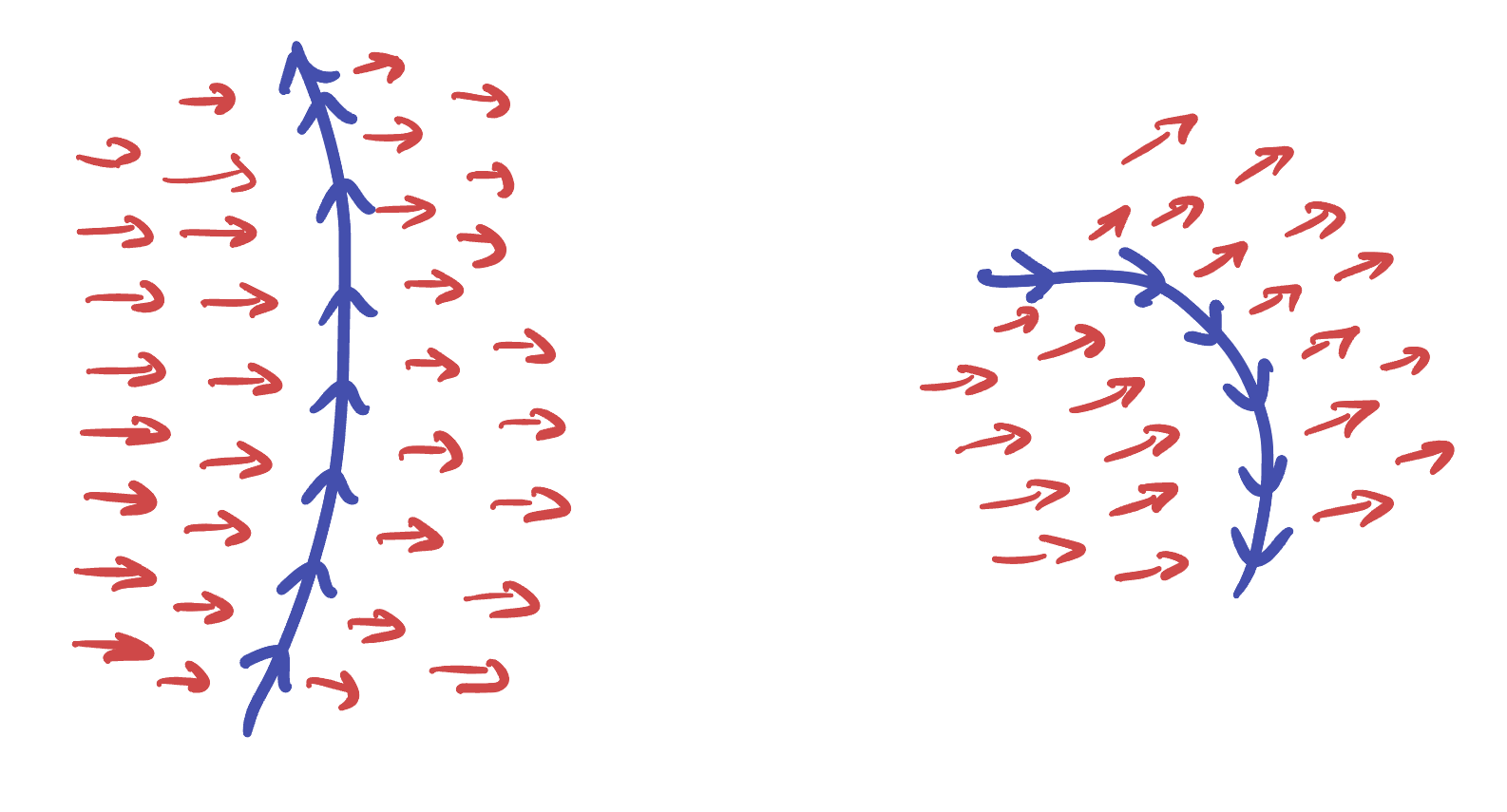
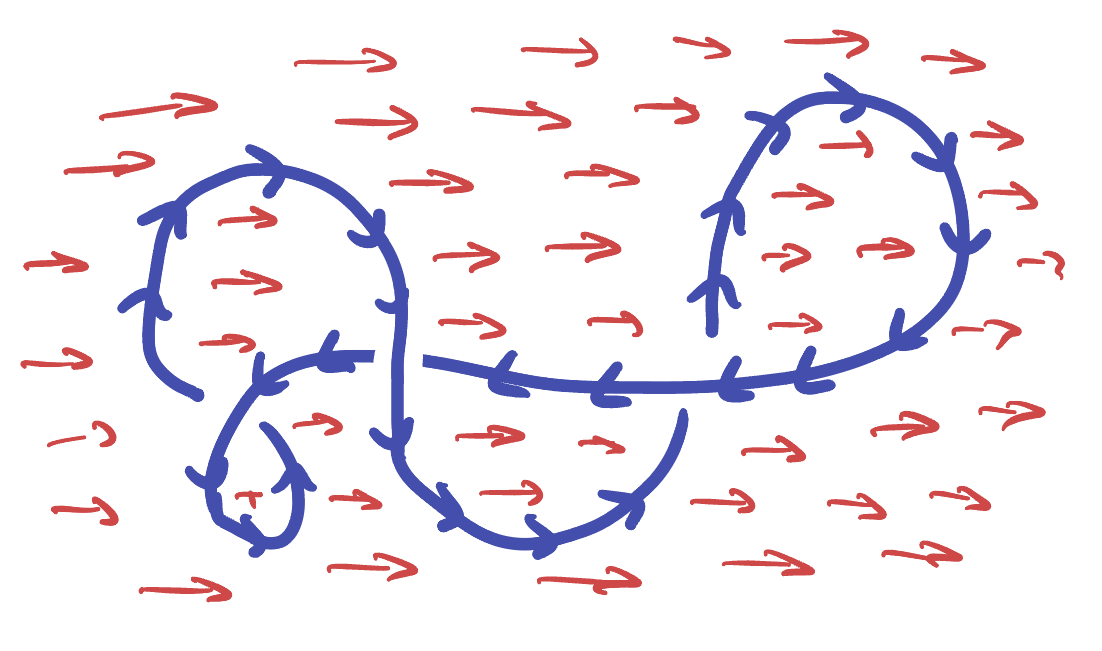
Circulation is defined given an oriented curve (that is, a curve with a specified direction for its parameterization) and a vector field. The goal is to measure whether the vector field’s net affect is to point along the direction of motion for the curve, or to point against the motion of the curve. We will call the former positive circulation and the latter negative circulation.

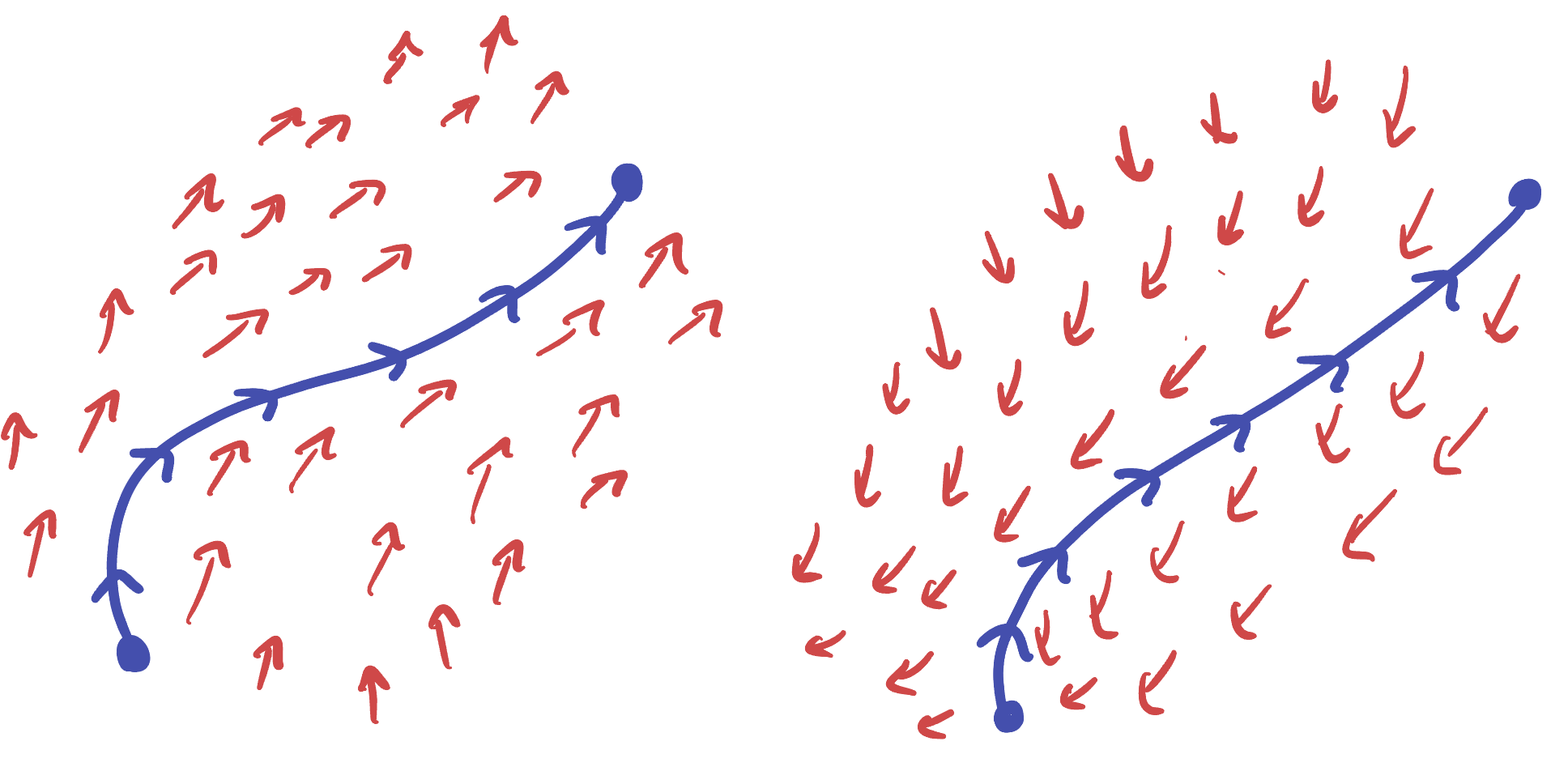The left vector field has positive circulation along the curve, whereas the right has negative.

A vector field has zero circulation along a curve if it overall neither aligns or anti-aligns on average. This can happen in several ways: perhaps it lines up with the curve half the time and opposes it the other half, or alternatively could simply be perpendicular to the curve at all times.

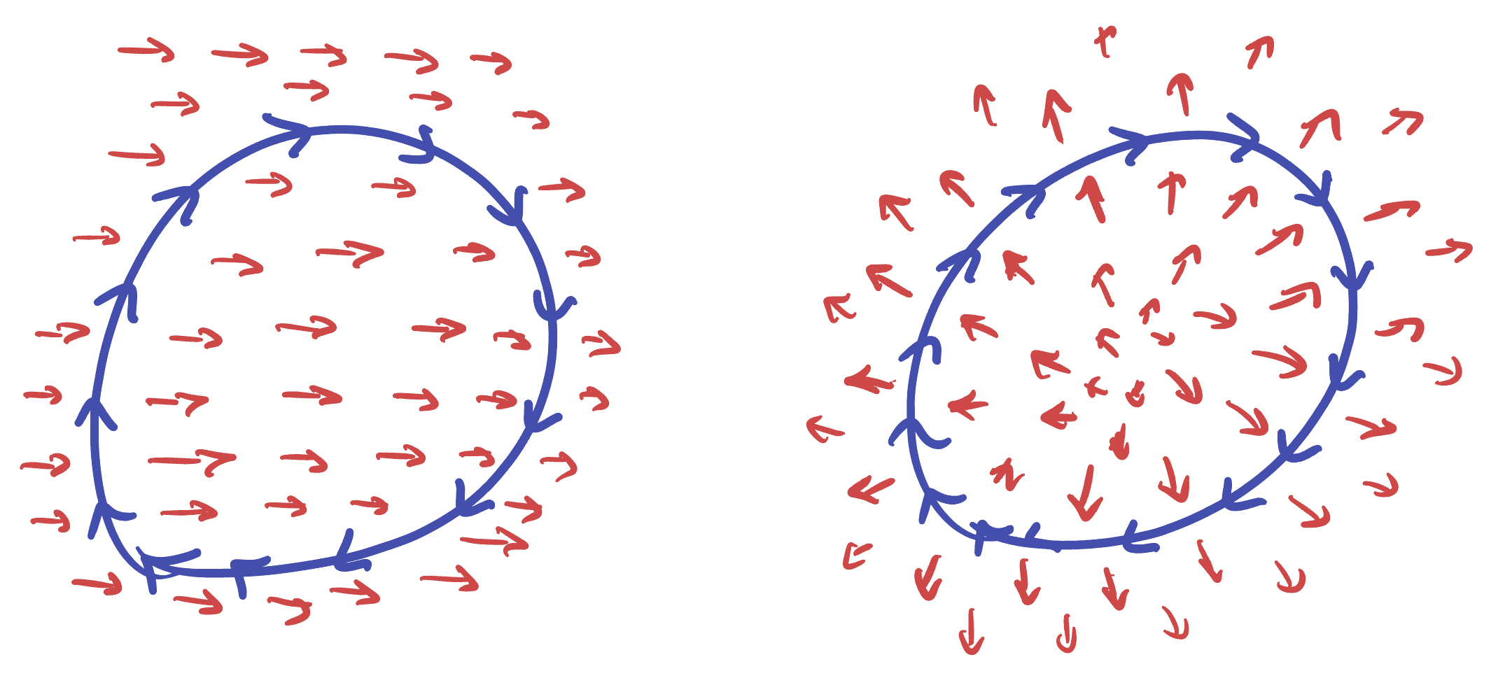These two vector fields have zero circulation around the curve.

We need to do some work now to turn this definition into a precise mathematical quantity. Since we are measuring a net affect along a curve, we can greatly simplify things by breaking down into two steps

• 1. Quantify how well a vector field aligns / anti-aligns with a curve at a point.
• 2. Get the net affect by adding these all up in a line integral along the curve.

Focusing on point (1), we can zoom in on a single point along our curve $p$ and reaching back deep into our memories from early in the course, notice that we actually already know how to compute the amount of $F$ pointing along our curve! It’s just the *component of $F$ in the direction tangent to the curve.

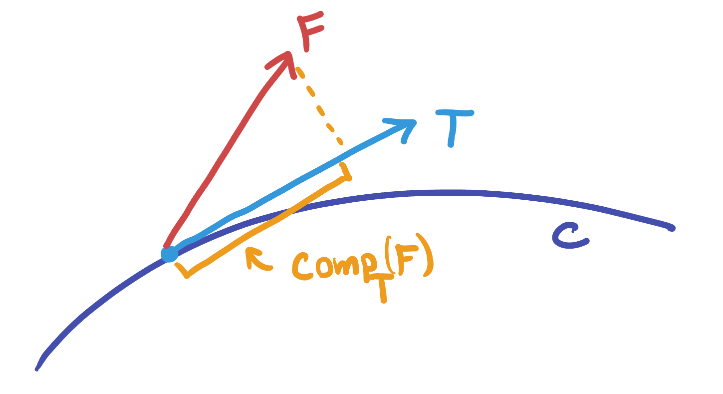
We can compute this by choosing any tangent vector $T$ pointing along the curve (in the direction of motion), and using a dot product

$${\mathrm{comp}}_T(F)=\frac{F\cdot T}{|T|}$$

Definition 19.1 (Circulation Integral) The circulation of a vector field $F$ along an oriented curve $C$ is defined as $${\int }_C{\mathrm{comp}}_T(F)ds={\int }_C\frac{F\cdot T}{|T|}ds$$ where $T$ is a choice of tangent vector to the curve

Now that we have a conceptual formula down, lets try to simplify it into something usable. Given a parameterization $\overrightarrow{c}(t)$ of our curve, at time $t$ we can choose the tangent vector to simply be the derivative ${\overrightarrow{c}}^{\prime }(t)$, and the vector field at that point is simply $\overrightarrow{F}(\overrightarrow{c}(t))$. This gives an explicit formula for the alignment at a point

$$\frac{\overrightarrow{F}(\overrightarrow{c}(t))\cdot {\overrightarrow{c}}^{\prime }(t)}{|{\overrightarrow{c}}^{\prime }(t)|}$$

This simplifes greatly inside of a line integral, because the definition of infinitesimal arclength also involves $|{\overrightarrow{c}}^{\prime }|$:

$${\int }_C\frac{\overrightarrow{F}(\overrightarrow{c}(t))\cdot {\overrightarrow{c}}^{\prime }(t)}{|{\overrightarrow{c}}^{\prime }(t)|}ds=\int \frac{\overrightarrow{F}(\overrightarrow{c}(t))\cdot {\overrightarrow{c}}^{\prime }(t)}{|{\overrightarrow{c}}^{\prime }(t)|}|{\overrightarrow{c}}^{\prime }(t)|dt=\int \overrightarrow{F}(\overrightarrow{c}(t))\cdot {\overrightarrow{c}}^{\prime }(t)dt$$

The norms cancel and we end up with a relatively simple integral: just the dot product of $F$ along the curve with the curve’s derivative! This form makes it easy to see how to compute such an integral so we record it for (much) future use as a theorem

Theorem 19.1 (Circulation Integral, in Usable Form) Given a vector field $F$ and parametric curve $c(t)$ for $t\in [a,b]$, the circulation integral can be computed via $${\int }_C{\mathrm{comp}}_T(F)ds={\int }_a^{b}F(c(t))\cdot c^{\prime }(t)dt$$

Let’s do a quick example to confirm this is an easy computation:

Example 19.1 Compute the circulation of $F=⟨xy,y+1⟩$ along the parabola $c(t)=(t,t^2)$ for $t\in [0,1]$.

We compute the vector field along the curve by simply subbing in the curves $x=t$, $y=t^2$ for $x,y$: $$F(c(t))=F(t,t^2)=⟨(t)(t^2),(t^2)+1⟩=⟨t^3,t^2+1⟩$$ Differentiating $c$ gives the tangent vector $$c^{\prime }(t)=⟨1,2t⟩$$ computing their dot product yields the integrand $$F(c(t))\cdot c^{\prime }(t)=⟨t^3,t^2+1⟩\cdot ⟨1,2t⟩=t^3+(t^2+1)2t=3t^3+2t$$ Integrating over the bounds gives the net circulation $${\int }_0^{1}3t^3+2tdt=\frac{3t^4}{4}+t^2{|}_0^1=\frac{3}{4}+1=\frac{7}{4}$$

If the curve $C$ consists of multiple piecewise components, one simply repeats this procedure for each component and adds the results, exactly as for a standard line integral.

Like many things in multivariable calculus, there are multiple notations for the circulation integral, suited to different purposes. In addition to the form we have right now ${\int }_a^{b}F(c(t))\cdot c^{\prime }(t)dt$, there is also a longer and a shorter notation in use. First, for the shorter one we can adopt the shorthand of $d\overrightarrow{s}$ for the infinitesimial displacement vector $$d\overrightarrow{s}={\overrightarrow{c}}^{\prime }(t)dt$$ much as we use $ds=|{\overrightarrow{c}}^{\prime }(t)|dt$ for infinitesimal distance. Substituting this into our integral gives the notation $${\int }_C\overrightarrow{F}\cdot d\overrightarrow{s}$$

Which is easy to unpack directly back to our other notation by substituting in the definition of $d\overrightarrow{s}$, and its conciseness is particularly helpful when doing long theoretical calculations where we aren’t necessarily immediately trying to compute the integral. On the other hand, one might also wish for an even more expanded notation than our original, that is amenable to directly plugging in for computation. One can come up with such a notation by expanding $F$ as $F=⟨P,Q⟩$ and writing out the dot product:

$$F\cdot c^{\prime }=⟨P,Q⟩\cdot ⟨x^{\prime },y^{\prime }⟩=P{x}^{\prime }+Q{y}^{\prime }$$

This is our integrand, and so we can rewrite the circulation as

$${\int }_C(P{x}^{\prime }+Q{y}^{\prime })=\int P{x}^{\prime }dt+Q{y}^{\prime }dt$$

using the shorthand that $x^{\prime }dt=dx$ and $y^{\prime }dt=dy$, this yields the memorable notation

$${\int }_C\overrightarrow{F}\cdot d\overrightarrow{s}={\int }_{C}Pdx+Qdy$$

We collect all these notations below in one place for future reference.

Definition 19.2 (Notation for Circulation Integrals) Given an oriented curve $c$ and a vector field $F$ we have several different notations for the circulation integral of $F$ along $c$: $$\mathrm{Circulation}={\int }_C{\mathrm{comp}}_{\overrightarrow{T}}(\overrightarrow{F})ds={\int }_C\overrightarrow{F}\cdot d\overrightarrow{s}={\int }_{C}Pdx+Qdy$$

19.2 Flux

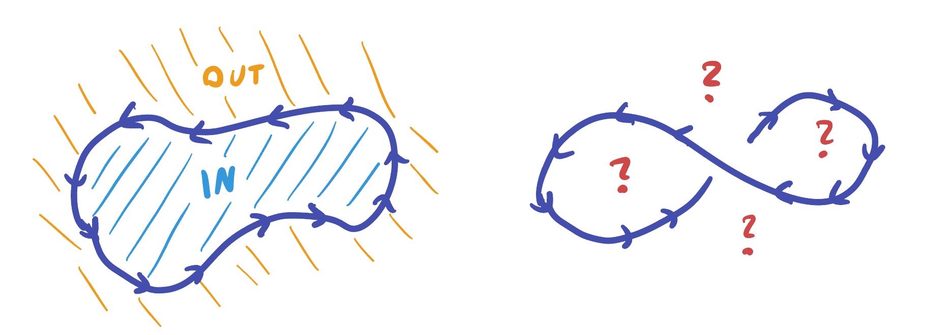
The story of flux through a curve is very similar to circulation, save one crucial detail. We are no longer interested in flow along the curve but rather flow through. We make the convention that if a curve is closed (which will be our most common use case) positive means net flow outwards and negative is flow inwards

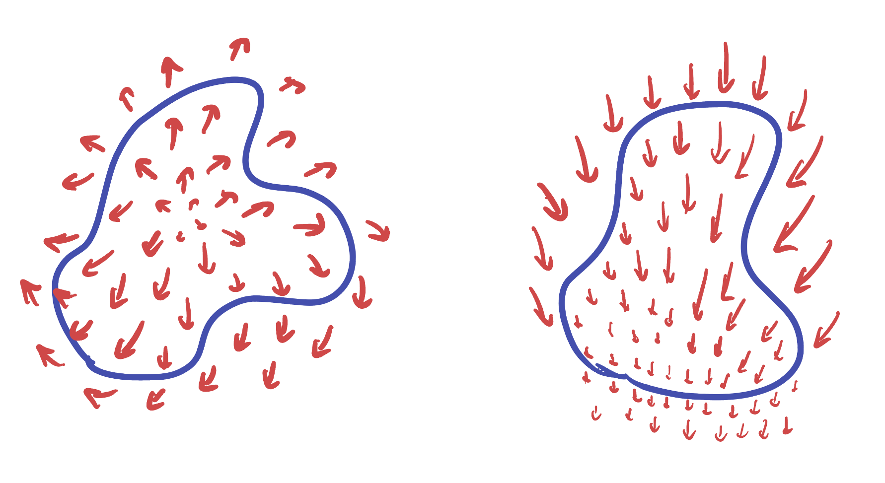Positive flux (left) as the vector field is flowing out of the curve at all points. Negative flux (right) even though the vector field is flowing overall downwards (into the curve at the top and out at the bottom), the inflow is greater than the outflow so the net flux is inwards.

And for an otherwise arbitrary parameterized curve, we will call positive flow from left to right along the direction of motion, and negative a flow from right to left (this matches with the above when a closed curve is parameterized counterclockwise - the math standard orientation).

The sign of flux has to do with the relative orientation of the curve and vector field. The left shows positive flux and the right negative flux, even though the vector field in both cases goes left to right.

Again its clear the net flow is going to be a line integral of the flow through a point, and so we need only compute it locally. Here sits the only change from our previous case: to measure outflow we are now concerned about the projection onto the normal instead of the tangent:

$${\mathrm{comp}}_N(F)=\frac{F\cdot N}{|N|}$$

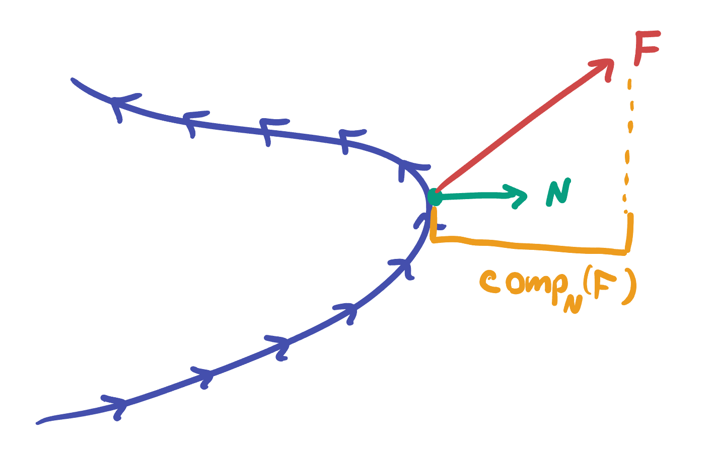
Definition 19.3 (Flux Integral) The flux of a vector field $F$ through an oriented curve $C$ is defined as $${\int }_C{\mathrm{comp}}_{\overrightarrow{N}}(\overrightarrow{F})ds={\int }_C\frac{\overrightarrow{F}\cdot \overrightarrow{N}}{|\overrightarrow{N}|}ds$$ where $N$ is a choice of normal vector to the curve at each point

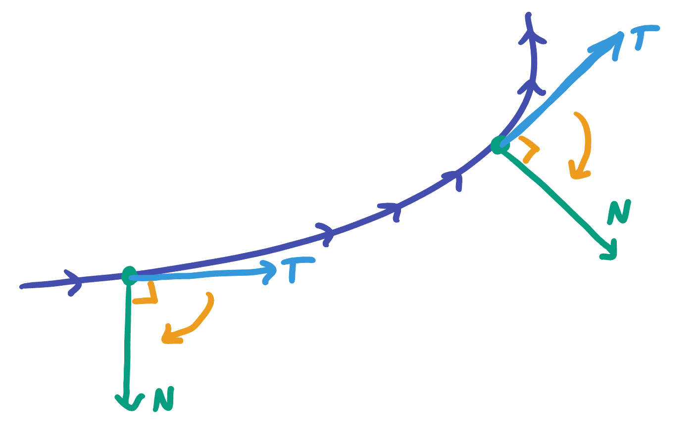
We again try to unpack this definition using an actual parameterization of the curve $c(t)=(x(t),y(t))$. Differentiation again gives us direct access to a tangent vector, and to get a correctly oriented normal vector we simply need to rotate this vector by $\pi /2$ clockwise:

How much of $F$ passes through the curve is quantified by the component of $F$ in the normal direction.

Such a rotation is accomplished by the transformation $(x,y)\mapsto (y,-x)$, which takes the tangent vector $c^{\prime }$ to the normal vector $n=⟨y^{\prime },-x^{\prime }⟩$. Using this normal vector in our calculation, we find

$${\mathrm{comp}}_n(F)=\frac{F\cdot ⟨y^{\prime },-x^{\prime }}{|⟨y^{\prime },-x^{\prime }⟩|}$$

This also simplifies greatly inside of the line integral, since the length of $n$ and the length of $c^{\prime }$ are equal to one another (one is just a rotation of the other, after all):

$${\int }_C\frac{F\cdot ⟨y^{\prime },-x^{\prime }⟩}{|⟨y^{\prime },-x^{\prime }⟩|}ds={\int }_C\frac{F\cdot ⟨y^{\prime },-x^{\prime }⟩}{|⟨y^{\prime },-x^{\prime }⟩|}|⟨x^{\prime },y^{\prime }⟩|dt$$ $$={\int }_{C}F\cdot ⟨y^{\prime },-x^{\prime }⟩dt$$

Actually performing this dot product for $F=⟨P,Q⟩$ suggests a further simplification that will make the formula even more memorable:

$$⟨P,Q⟩\cdot ⟨y^{\prime },-x^{\prime }⟩=P{y}^{\prime }-Q{x}^{\prime }$$

This is itself just a cross product!

$$P{y}^{\prime }-Q{x}^{\prime }=\left|\begin{array}{cc}P& Q\\ x^{\prime }& y^{\prime }\end{array}\right|=⟨P,Q⟩\times ⟨x^{\prime },y^{\prime }⟩=F\times c^{\prime }$$

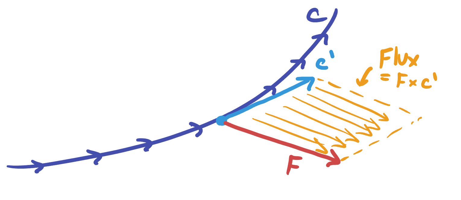This has a nice interpretation: this parallelogram is made of many parallel copies of $F$ infinitesimally translated along $c^{\prime }$: so its area truly is capturing the amount of $F$ flowing through $c$ along this segment of arc.

In addition to being a memorable picture, this new formula lends itself directly to computation, so let’s record it in a box and do an example

Theorem 19.2 Given a vector field $F$ and parametric curve $c(t)$ for $t\in [a,b]$, the flux integral can be computed via $${\int }_C{\mathrm{comp}}_N(F)ds={\int }_a^{b}F(c(t))\times c^{\prime }(t)dt$$

Example 19.2 Compute the flux of $F=⟨x+y,y⟩$ through the unit circle (oriented counterclockwise).

We start by writing down this standard parameterization $c(t)=(\cos t,\sin t)$ for $t\in [0,2\pi ]$. Then compute $c^{\prime }(t)=⟨-\sin (t),\cos (t)⟩$ and $F$ along the curve $$F(c(t))=F(\cos t,\sin t)=⟨\cos (t)+\sin (t),\sin (t)⟩$$

Taking the cross product gives the integrand

$$F\times c^{\prime }=\left|\begin{array}{cc}\cos (t)+\sin (t)& \sin (t)\\ -\sin (t)& \cos (t)\end{array}\right|=(\cos t+\sin t)\cos t+{\sin }^{2}t$$ $$={\cos }^{2}t+\cos t\sin t+{\sin }^{2}t=1+\cos t\sin t$$

Integrating then directly gives the flux $${\int }_0^{2\pi }1+\cos (t)\sin (t)dt=2\pi +0=2\pi$$

For consistency we can also seek better, more memorable notations for the flux integral like we did for circulation. The integrand $F(c(t))\times c^{\prime }(t)dt$ immediately collapses to $\overrightarrow{F}\times d\overrightarrow{s}$ under our shorthand $d\overrightarrow{s}={\overrightarrow{c}}^{\prime }(t)dt$, and the longer, ‘plug it in form’ is deducible from our computations above $Pdy-Qdx$

Definition 19.4 (Notation for Flux Integrals) Given an oriented curve $c$ and a vector field $F$ we have several different notations for the flux integral of $F$ through $c$: $$\mathrm{Flux}={\int }_C{\mathrm{comp}}_N(F)ds={\int }_C\overrightarrow{F}\times d\overrightarrow{s}={\int }_{C}Pdy-Qdx$$

19.3 Circulation and Flux in 3 Dimensions

The defintiion of circulation remains unchanged in three dimensions, as it still makes perfect sense to try and measure how much a 3D vector field aligns with a 3D curve. Indeed, the formula remains the same, integrating the tangential component along the curve, and the entirety of the previous discussion goes through just with one added coordinate

Definition 19.5 (Circulation in 3D) Given a vector field $\overrightarrow{F}=⟨P,Q,R⟩$ and a parametric curve $c(t)=(x(t),y(t),z(t))$, the net circulation of $F$ along $c$ is given by the integral

$${\int }_C{\mathrm{comp}}_T(F)ds={\int }_C\overrightarrow{F}\cdot d\overrightarrow{s}={\int }_{C}Pdx+Qdy+Rdz$$

Example 19.3 Compute the circulation of $F=⟨xy,y+z,z^2⟩$ along the circle $c(t)=⟨\cos (t),\sin (t),1⟩$.

Again we find $F$ along the curve as $$F(c(t))=F(\cos t,\sin t,1)=⟨\cos t\sin t,\sin t+1,1^2⟩$$ and the tangent vector to the curve as $$c^{\prime }(t)=⟨-\sin t,\cos t,0⟩$$ Their dot product is the integrand $$⟨\cos t\sin t,\sin t+1,1^2⟩\cdot ⟨-\sin t,\cos t,0⟩=-\cos t{\sin }^{2}t+{\sin }^{2}t+\sin t+0$$ And integrating this over the curve yields the circulation

$${\int }_0^{2\pi }-\cos t{\sin }^{2}t+{\sin }^{2}t+\sin tdt=-0+\pi +0=\pi$$

(While it won’t be relevant to our course, this definition continues to make sense in all dimensions, via the exact same formula).

Turning to flux, it perhaps comes as no surprise that things must change. There are both conceptual and formulaic problems with trying to naively apply our earlier formulation:

• 1. The formula involves a cross product, and this changes from a scalar quantity to a vector quantity in 3 dimensions, but we still want our overall integral to be a scalar.
• 2. Flux is supposed to measure the flow through something. But a curve does not separate two regions in 3D space like it does in the plane, so there’s no natural inside and outside.

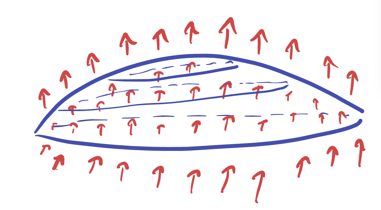
Both of these problems are fixed by realizing that the natural notion of a flux integral in three dimensions needs to be a surface integral instead of a line integral. This is the only change to the definition: flux is still the normal component of the vector field

Definition 19.6 (Flux Integrals in 3D) The flux of a vector field $\overrightarrow{F}$ through a surface $S$ is given by $${\iint }_S{\mathrm{comp}}_N(F)dS$$ where $N$ is a normal vector to the surface, and $dS$ the infinitesimal surface element.

Using our previous experience, we should try to simplify this formula a bit, hoping that any square roots hidden in the definition of the normal component cancel out with square roots in the definition of $dS$. To be explicit about this, we’ll write this down for the case that $S$ is the graph of a function $z=g(x,y)$ like we considered previously. A short review here is helpful: we found the surface area element $dS$ by first finding two tangent vectors to the surface at a point

$$T_x=⟨1,0,g_x⟩T_y=⟨0,1,g_y⟩$$

and then finding the area of the parallelogram they span by taking the magnitude of their cross product

$$\mathrm{Area}=|T_x\times T_y|=\sqrt{1+g_x^2+g_y^2}$$

For us now, its very convenient to note that before taking this magnitude, the cross product is itself a normal vector to our surface (in fact, it is the upward facing normal)

$$N=T_x\times T_y=⟨-g_x,g_y,1⟩$$

If we use this normal vector, the simplifications that happen in our formula become more apparent:

$${\mathrm{comp}}_N(F)dS=\frac{F\cdot N}{|N|}dS=\frac{F\cdot N}{|N|}|N|dxdy=F\cdot Ndxdy$$

This gives an easy formula to calculate the flux integral over a surface $z=g(x,y)$, very analogous to the case one dimension down

Theorem 19.3 (Flux Integrals in 3D) The flux of the vector field $F$ through a surface $S$ of a graph $z=g(x,y)$ can be computed as $${\iint }_S\overrightarrow{F}\cdot Ndxdy$$ Where $N=⟨-g_x,g_y,1⟩$ is the upward facing normal.

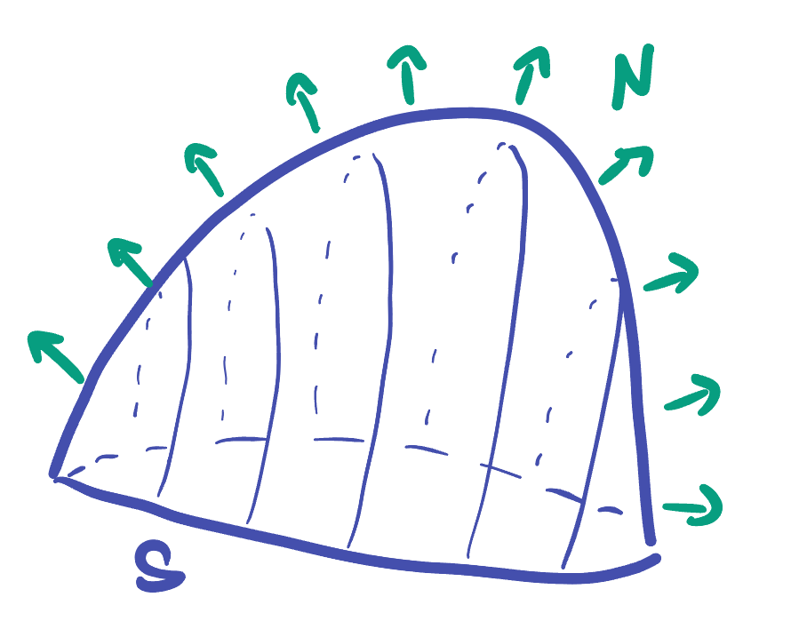The upward facing normal.

At this point an example is in order

Example 19.4 Calculate the flux of $\overrightarrow{F}=⟨x,z,1⟩$ through the surface $z=1-x^2+y^2$ for $z\ge 0$, with an upward pointing normal vector.

We can compute the vector field on our surface by substituting $z=1-x^2-y^2$ into $\overrightarrow{F}$: $$F(x,y,z)=F(x,y,1-x^2-y^2)=⟨x,1-x^2-y^2,1⟩$$ Computing the normal vector, $z_x=-2x$, $z_y=-2y$ and $$N=⟨2x,2y,1⟩$$

This gives the integrand $$F\cdot N=⟨x,1-x^2-y^2,1⟩\cdot ⟨2x,2y,1⟩=2x^2+2y(1-x^2-y^2)+1$$ $$=2x^2-2x^{2}y-2y^3+2y+1$$

The flux integral is then just this over the domain, which is the unit circle $R$ in the $xy$ plane (what we get from setting $z=1-x^2-y^2$ and $z=0$ equal to one another). $${\iint }_{R}2x^2-2x^{2}y-2y^3+2y+1dxdy$$

This integral is best computed by converting to polar coordinates.

This same idea works for general parametric surfaces with little change: if we write $S$ using a parameterization $$r(u,v)=(x(u,v),y(u,v),z(u,v))$$ we can find tangent vectors $T_u$ and $T_v$ just as before $$T_u={\partial }_{u}r=⟨x_u,y_u,z_u⟩T_v={\partial }_{v}r=⟨x_v,y_v,z_v⟩$$ and define the normal vector $N=T_u\times T_v$.

Theorem 19.4 (Flux Integrals over Parametric Surfaces) The flux of the vector field $F$ through a surface $S$ parameterized by $r=(x(u,v),y(u,v),z(u,v))$ is $${\iint }_S\overrightarrow{F}\cdot Ndudv={\iint }_S\overrightarrow{F}\cdot (T_u\times T_v)dudv$$

A final note: the most common use case (in physics, and electrical engineering) involves $S$ being a closed surface, where like for closed curves, we will take the default to mean outward facing normal. When our surface is made of multiple pieces, we’ll need to make sure that we give each piece the correct normal vector (sometimes this will have to be the downwards facing normal vector)

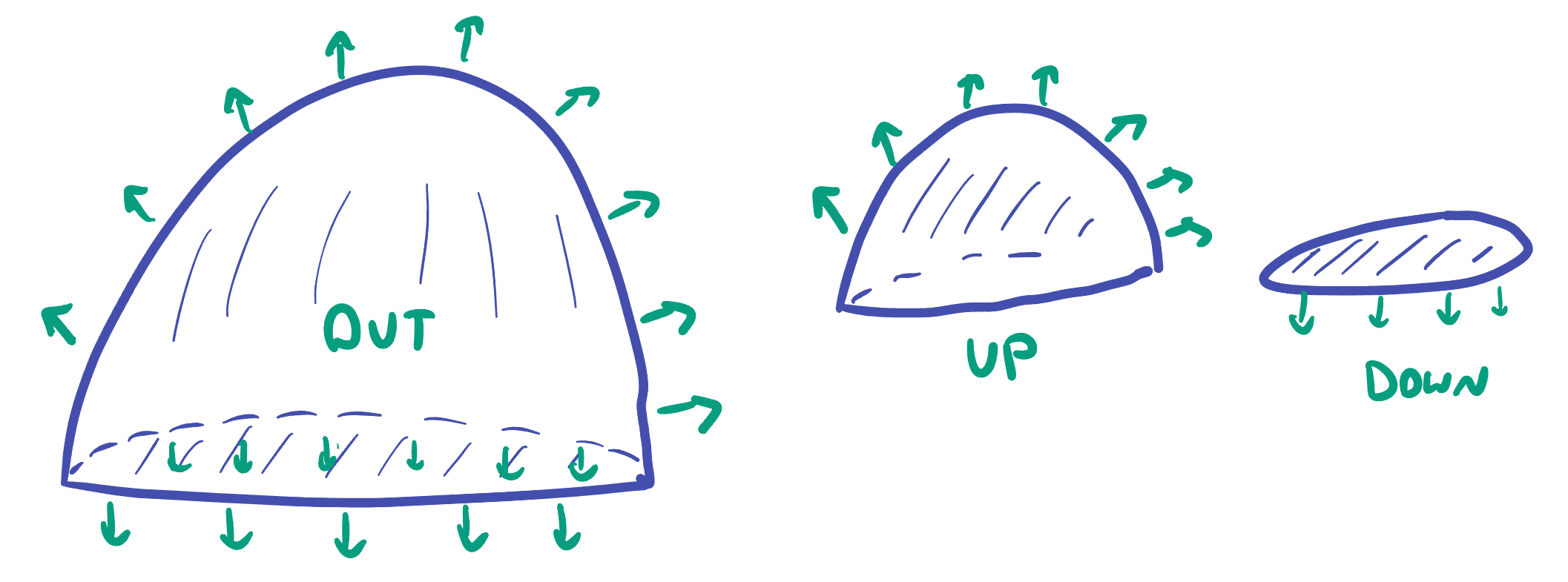Making sure to get the outward normal everywhere means drawing a picture and figuring out which pieces need upwards vs downwards normals.

Example 19.5 Calculate the flux of $\overrightarrow{F}=⟨x,z,1⟩$ through the closed surface bounded by $z=1-x^2+y^2$ for $z\ge 0$ and the unit disk in the $z=0$ plane, with outwards facing normal.

The top half of this problem is exactly the same integral as in the previous example. To do the bottom half, we deal with the unit disk $D$ in the $xy$ plane. To make sure the entire normal vector is pointed outward we actually need the downwards normal here (since the upper half of the surface used the upwards normal).

So, for this second integral $N=⟨0,0,-1⟩$ and $dS=dxdy$ (since we are in a piece of the $xy$ plane). Computing the vector field on this region is as simple as substituting $z=0$, giving $F=⟨x,0,1⟩$. Taking the dot product gives $$F\cdot N=⟨x,0,1⟩\cdot ⟨0,0,-1⟩=-1$$ and so the surface integral for the bottom half of the surface becomes $${\iint }_R(-1)dxdy$$

This is just $-1$ times the area of the unit disk, or $-\pi$.