$$$$

17  Line & Surface Integrals

We’ve learned so far to integrate multivariate functions over a line or over regions in ${\mathbb{R}}^2$ or ${\mathbb{R}}^3$. Here we extend our knowledge to consider integrals over a curve or a surface in space. Such integrals appear in many mathematical and physical contexts, and in particular turn out to be rather important in our final unit, dealing with vector fields.

17.1 Line Integrals

A better name for this object would be a curve integral as the goal is to allow the integration of a multivariable function $f$ over some general curve $C$. We already know how to do this if $C$ is a straight line parallel to the $x$ or $y$ axes, as this is just a slice, representing the net area above that slice, or the total amount of $f$ on that slice:

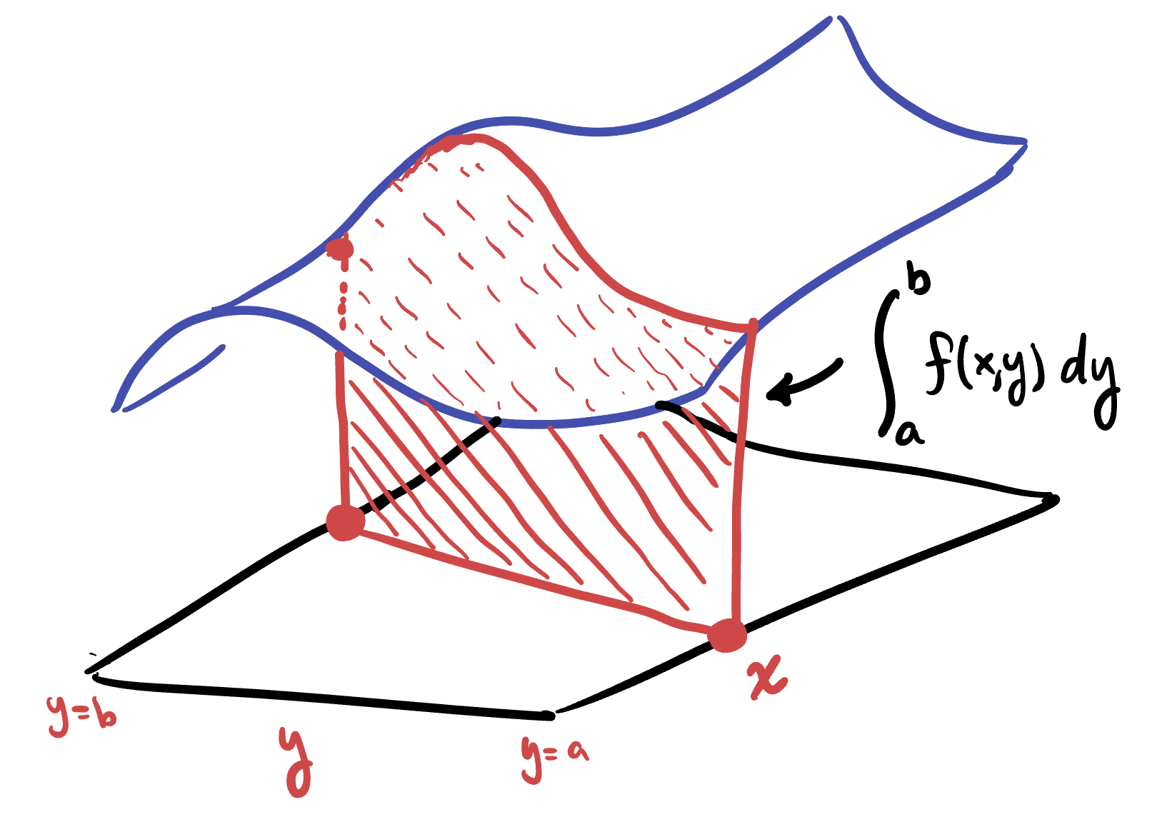
This picture caries over directly when $C$ is an arbitrary curve. The area under $f$ above the curve $C$ (or the total amount of $f$ along $C$, depending on your interpretation) is the line integral over $C$

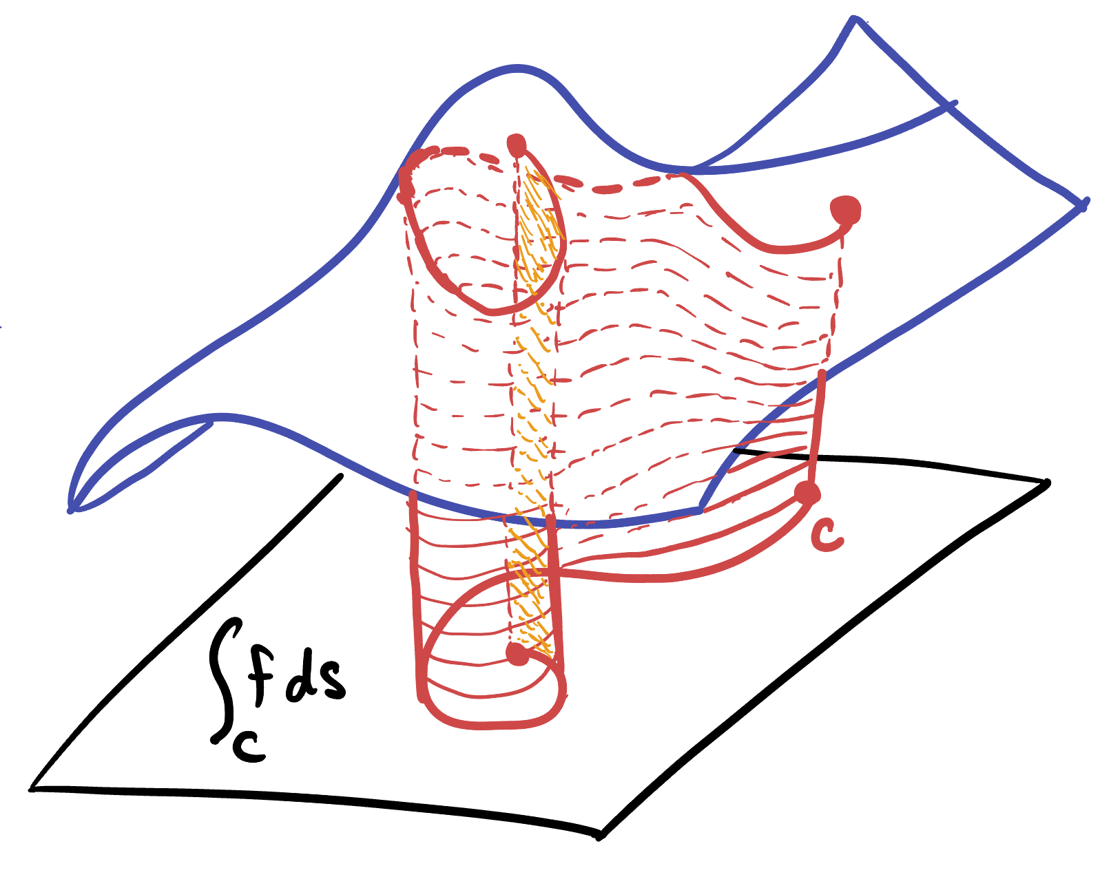
We can denote the domain $C$ as a subscript just like we do for double and triple integrals, and write

$${\int }_{C}fds$$

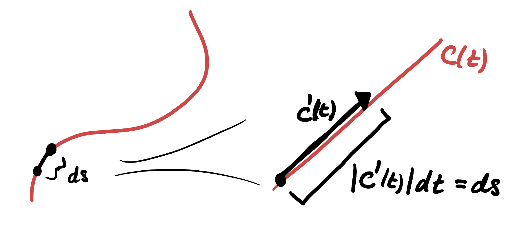
Where $ds$ represents an infinitesimal bit of arclength along the curve. When $C$ is a closed curve one may optionally modify the integral sign to denote this, writing ${\oint }_{C}fds$. Our first goal is to try and figure out how to compute this in terms of integrals we know how to do. First: recall that we can represent a curve $C$ by parameterizing it, writing it as the image of a function $c(t)=(x(t),y(t))$ in the plane, or $c(t)=(x(t),y(t),z(t))$ in 3 dimensions. We saw back in the chapter on curves how to express a small bit of arclength along a parametric curve:

$$ds=\sqrt{d{x}^2+d{y}^2}=\sqrt{\frac{d{x}^2}{d{t}^2}d{t}^2+\frac{d{y}^2}{d{t}^2}d{t}^2}=\sqrt{x^{\prime }(t{)}^2+y^{\prime }(t{)}^2}dt=\parallel c^{\prime }(t)\parallel dt$$

To evaluate a function $f(x,y,z)$ along the curve $c(t)=(x(t),y(t))$, we simply plug the curve into the function. This gives a concrete quantity to integrate:

$${\int }_{C}fds={\int }_a^{b}f(c(t))\parallel c^{\prime }(t)\parallel dt$$

Note the simplest line integrals are just when $f=1$. This is the integral just adding up the infinitesimal arclengths ${\int }_{C}ds=\int \parallel c^{\prime }\parallel dt$. We already met this integral long ago - this gives the arclength of the curve!

Example 17.1 The slices we have been computing are special cases of line integrals: for a fixed $x=a$ we can parameterize a slice in the $y$ direction by the curve $c(t)=(x,t)$ which has velocity $c^{\prime }=(0,1)$ and speed $\parallel c^{\prime }\parallel =1$, so arclength $ds=\parallel c^{\prime }\parallel dy=1dy$. Plugging our curve into the function yields $f(c(t))=f(x,t)$ and thus an integral $$\int f(x,t)dt$$ The variable has a different name (because we decided to parameterize our curve with $t$) but this is nothing other than the integral in the $y$ direction, holding $x$ fixed!

Example 17.2 Find ${\int }_{C}xyds$ for $C$ the diagonal of the unit square going from $(0,0)$ to $(1,1)$.

Example 17.3 Evaluate ${\int }_C(2+x^{2}y)ds$ for $C$ the top half of the unit circle parameterized counterclockwise.

Example 17.4 Evaluate ${\oint }_C{x}^{2}ds$ for $C$ the circle of radius $2$, traversed clockwise.

This tells us what to do anytime we can write $C$ as a differentiable curve: but what if we can’t? Sometimes a curve $C$ might be piecewise, and has a corner where the edges join up. In this case, we evaluate the line integral by doing each segment of the curve separately, and adding the results:

$${\int }_{C_1\cup C_2}fds={\int }_{C_1}fds+{\int }_{C_2}fds$$

We just have to be sure to parameterize the two curves so that $C_1$ ends where $C_2$ starts, so that together they continuously trace the entire curve.

Example 17.5 Find the line integral of $x$ along the curve $C$ which traces out the triangle with vertices $(0,0)$, $(1,0)$ and $(0,1)$, starting at the origin and going clockwise.

We break this into three curves: $$c_1(t)=(t,0)c_2(t)=(1-t,t)c_3(t)=(0,1-t)$$ Each is segment is traced from $t=0$ to $t=1$. We then just compute the line integral along each and add up the results.

Its no difficulty to generalize this to doing integrals along space curves instead of in the plane:

Example 17.6 Compute the line integral ${\int }_{C}fds$ for $f(x,y,z)=y\sin z$ and $C$ the helix $x=\cos t$, $y=\sin t$ and $z=t$ for $t\in [0,2\pi ]$.

17.2 Surface Integrals

We are now interested in extending this notion to integrals over a surface instead of a curve. If that surface $S$ is a 2D region inside of the $xy$ plane, we already know how to do this: its just the double integral ${\iint }_{S}fdA$, where $dA$ is an infinitesimal piece of area on the plane. So, what we are interested in here instead is when $S$ is a surface in 3 dimensional space and $f(x,y,z)$ is a scalar function on 3 dimensional space

These integrals will add up the total amount of $f$ which lies on the surface $S$. This is useful for many things: if $f$ is a density this gives the mass of the object. If $f$ is a charge density this would give the total charge on the surface: a computation that is useful inside of batteries, where the anode and cathode may be tightly coiled surfaces. These integrals can also be used to help find the average value of a function: dividing the surface integral of $f$ over $S$ by the surface area of $S$. We will denote such an integral as

$${\iint }_{S}fdS$$

Where we think of $dS$ as an infinitesimal piece of surface area. A lot of the work in computing surface integrals is just finding the right form for $dS$ to use, to convert int into a double integral we know how to do. So we begin by looking at some special cases: we actually know how to write the infinitesimal areas on a cylinder or sphere from our work with coordinates!

The Surface of a Cylinder

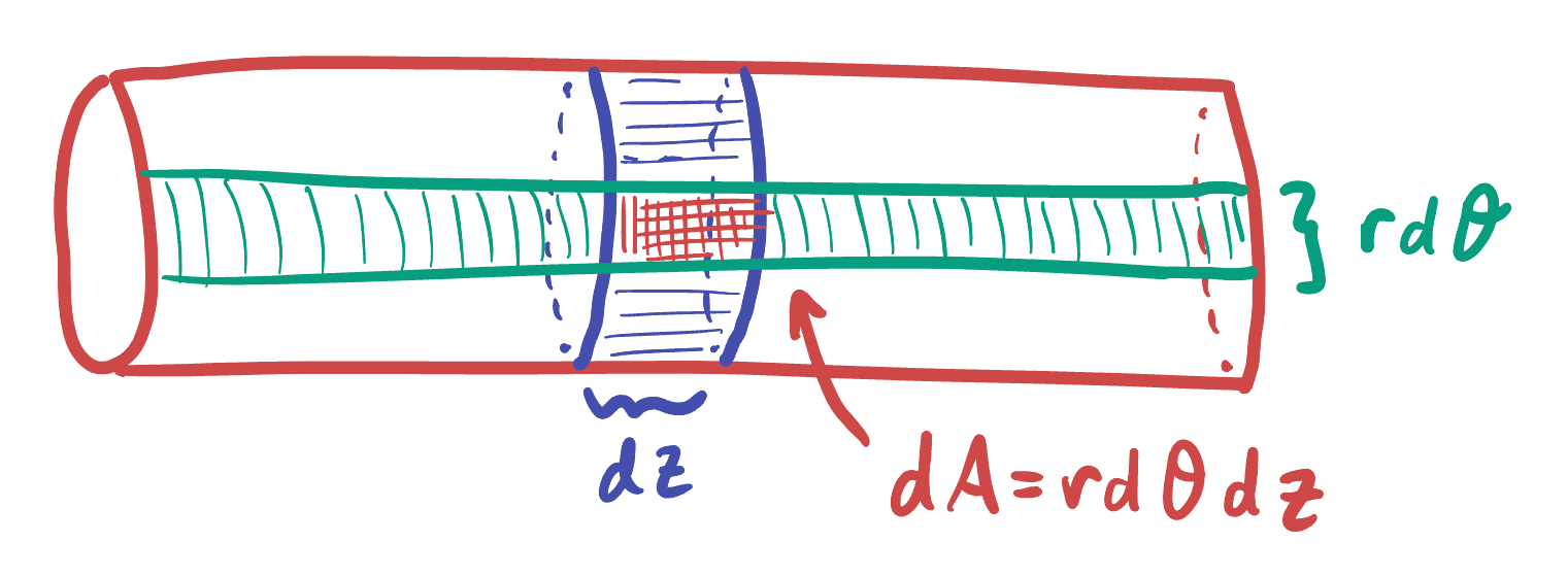
In cylindrical coordinates we convert two of $x,y,z$ to polar $r,\theta$ and leave the other alone. The resulting volume element was $$dV=dzrdrd\theta$$

We can use this to find the area element on a cylinder, realizing this simply means that $r$ is held fixed and $z,\theta$ are allowed to vary:

Definition 17.1 The area element along a cylinder of fixed radius $r$ is $$dS=rd\theta dz$$

Thus, to compute a surface integral of $f$ on a portion of a cylinder, we can convert $f$ to cylindrical coordinates and then use the cylinders’s area element:

Example 17.7 Compute ${\iint }_S{x}^{3}dS$$ for $S$ the cylinder of radius 2 centered on the $z$-axis between $z=1$ and $z=3$.

Here $x=2\cos \theta$ $y=2\sin \theta$ and $z$ remains the same, giving $dS=2d\theta dz$ and $x^3=(2\cos \theta {)}^3=8{\cos }^3\theta$. The bounds on the cylinder are $0\le \theta \le 2\pi$ and $z\in [1,3]$. Putting this all together gives $${\iint }_S{x}^{3}dS={\int }_1^3{\int }_0^{2\pi }8{\cos }^3\theta d\theta dz$$

This is a double integral we can easily evaluate, using the trick ${\cos }^3\theta =(1-{\sin }^2\theta )\cos \theta$ and a $u$-substitution.

Example 17.8 Compute ${\iint }_{S}xdS$ for $S$ the cylinder of radius 1 centered on the $x$ axis from $x=0$ to $x=2$.

Here the cylinder is along the $x$ axis so we instead have $y,z$ being the polar coordinates. The cylinders bounds are $\theta \in [0,2\pi ]$ and $x\in [0,2]$, with $dS=d\theta dx$ since $r=1$. Plugging all this in yields

$${\iint }_{S}xdS={\int }_0^2{\int }_0^{2\pi }xdxd\theta$$

The Surface of a Sphere On a sphere we already have spherical coordinates for which we computed a nice volume element $$dV={\rho }^2\sin \varphi d\rho d\varphi d\theta$$

If we wish to look at the area of a sphere we just need to fix $\rho$ to some constant value (its radius), and then consider only small changes in $\varphi$ and $\theta$ (we are not changing $\rho$ as we wish to stay on the surface!)

Definition 17.2 The infinitesimal area element on a sphere of radius $r$ is $$dS=r^2\sin \varphi d\varphi d\theta$$

Thus, to compute a surface integral of $f$ on a portion of a sphere, we can convert $f$ to spherical coordinates and then use the sphere’s area element:

Example 17.9 Compute ${\iint }_{S}zdS$ for $S$ the upper hemisphere of the sphere of radius $2$.

In spherical coordinates $z=\rho \cos \varphi$, and here the radius is fixed at $2$ so $z=2\cos \varphi$. The spherical coordinate bounds for the upper hemisphere have $\varphi \in [0,\pi /2]$ and $\theta \in [0,2\pi ]$, so plugging these in with the area element $dS=4\sin \varphi d\varphi d\theta$ yields

$${\iint }_{S}zdS={\int }_0^{2\pi }{\int }_0^{\pi /2}(2\cos \varphi )(4\sin \varphi )d\varphi d\theta =8{\int }_0^{2\pi }{\int }_0^{\pi /2}\cos \varphi \sin \varphi d\varphi d\theta$$

This integral is easily evaluated with a $u$-sub $u=\sin \varphi$.

Example 17.10 Compute ${\iint }_S(x^2+y^2+z^2)dS$ for $S$ the sphere of radius 3 centered at the origin.

The Graph of a Function

What about when our surface isnt something simple like this that we already know the answer to? Let’s start with the case that our surface is the graph of a function $z=g(x,y)$.

How do we describe an infinitesimal area element on this surface? Recalling back to our earlier study of functions and their graphs, we can easily find two tangent vectors to our graph by writing it as a parametric surface $$(x,y,g(x,y))$$ and then taking the partial derivatives. This gives a vector $v_x$ in the $x$ direction and $v_y$ in the $y$ direction

$$v_x=\frac{\partial }{\partial x}(x,y,g(x,y))=⟨1,0,g_x⟩v_y=\frac{\partial }{\partial y}(x,y,g(x,y))=⟨1,0,g_y⟩$$

These two vectors span an infinitesimal parallelogram, whose area is the area element we seek. How do we find the area of a small parallelogram again? The cross product! Thus, the area element is simply $$dS=\parallel v_x\times v_y\parallel dxdy$$

Computing this cross product and taking the magnitude gives our answer

$$v_x\times v_y=\left|\begin{array}{ccc}i& j& k\\ 1& 0& g_x\\ 0& 1& g_y\end{array}\right|=i(-g_x)-j(g_y)+k(1)=⟨-g_x,g_y,1⟩$$ $$\parallel v_x\times v_y\parallel =\sqrt{(-g_x{)}^2+(-g_y{)}^2+1^2}=\sqrt{1+g_x^2+g_y^2}$$

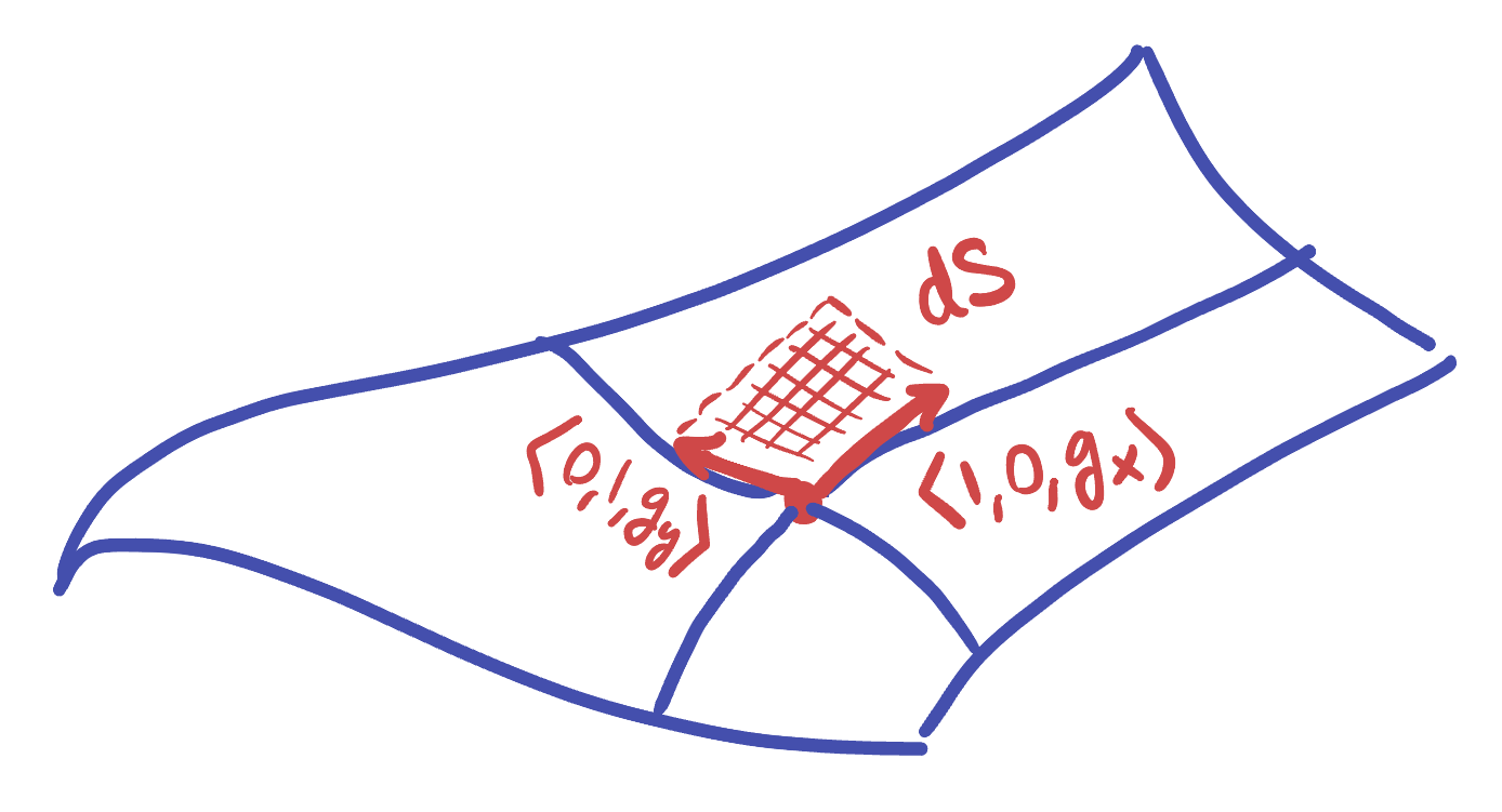
Definition 17.3 The area element along the graph of a function $z=g(x,y)$ is given by $$dS=\sqrt{1+g_x^2+g_y^2}dxdy$$

This gives us a means to evaluate surface integrals along such objects: we simply evaluate $f$ at points along the graph, and integrate with respect to this $dS$.

Example 17.11 Find the area of the paraboloid $z=x^2+y^2$ that lies below the plane $z=9$.

Example 17.12 Find ${\iint }_{S}ydS$ for $S$ the surface $z=x+y^2$ for $0\le x\le 1$ and $0\le y\le 2$.

Ans: $\frac{13\sqrt{2}}{3}$.

Just like for Line Integrals, surface integrals can be computed over regions bounded by two or more surfaces joined together by computing each part separately and adding the results:

Example 17.13 Let $S$ denote the closed surface defined by $z=2-x^2-y^2$ and the plane $z=1$. Compute the surface integral ${\iint }_{S}x+zdS$$

General Surface Integrals

The cases above actually cover many useful examples, so we will not often need the general case. But we’ve come so far we might as well spell it out precisely. Let’s say we have a surface $S$ in space described by a parametric equation $r(u,v)=(x(u,v),y(u,v),z(u,v))$. Its easy to evaluate a scalar function $f(x,y,z)$ on the surface, we just plug in this parameterization $$f(r(u,v))=f(x(u,v),y(u,v),z(u,v))$$

To get an infinitesimal surface area element, we can follow the trick that worked for graphs: if we can find two tangent vectors at a point we can find the area of the infintiesimal parallelogram they span using the cross product.

Here the tangent vectors are the $u$ and $v$ derivatives of the parameterization

$$r_u=\frac{\partial r}{\partial u}=⟨\frac{\partial x}{\partial u},\frac{\partial y}{\partial u},\frac{\partial z}{\partial u}⟩r_v=\frac{\partial r}{\partial v}=⟨\frac{\partial x}{\partial v},\frac{\partial y}{\partial v},\frac{\partial z}{\partial v}⟩$$

The normal vector to the surface at this point is the cross product $n=r_u\times r_v$ and its magnitude is the infinitesimal area element:

$$dS=\parallel r_u\times r_v\parallel dudv$$

This converts everything into an explicit double integral

$${\iint }_{S}fdS={\iint }_{D}f(r(u,v))\parallel r_u\times r_v\parallel dudv$$

Where $D$ is the domain of the parameterization (its $u$ bounds and $v$ bounds).

Example 17.14 Compute ${\iint }_{S}xyzdS$ for $S$ the cone parameterized by $x=u\cos v$, $y=u\sin v$ and $z=u$ for $u\in [0,1]$ and $v\in [0,2\pi ]$.

Example 17.15 Compute ${\iint }_S{x}^2+y^{2}dS$ for $S$ the surface with parameteric equation $r(u,v)=(2uv,u^2-v^2,u^2+v^2)$ where $(u,v)$ lies in the unit disk $u^2+v^2\le 1$.

17.3 Video Resources

17.3.1 Line Integrals

17.3.2 Surface Integrals