11 Extrema
We’ve developed some powerful tools for working with multivariable functions: we can take their partial derivatives, directional derivatives, and understand the relationship between the gradient and their level sets. Our next goal is to put this knowledge to work and learn how to find maximal and minimal values. This is a critical skill in real world applications, where we are looking to maximize efficiency, or minimize cost.
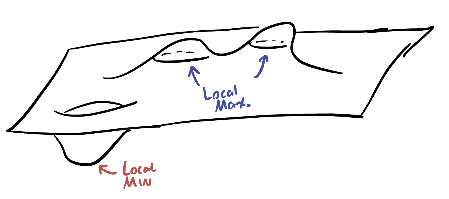
Definition 11.1 (Local Extrema) An extremum is a catch-all word for a maximum or a minimum (its an extreme value, meaning either largest or smallest). A local minimum is a occurs at a point \(p=(a,b)\) if the value of the function \(f(x,y)\) is always greater than or equal to \(f(a,b)\), when \(x\) is near \(a\) and \(y\) is near \(b\). Analogously, a local maximum occurs at \((a,b)\) if \(f(x,y)\leq f(a,b)\) for all \((x,y)\) near \((a,b)\).
In this section we will mainly be concerned with how to find local maxima and minima, though in optimization we will often be after the maximal value or minimal value of the function overall. These global maxima or minima are often just the largest or smallest of the local extrema, so our first step will be to find the local counterparts, then sort through them.
How can we find an equation to specify local extrema? In calculus I we had a nice approach using differentiation: at a local max or min a function is neither increasing nor decreasing so its derivative is zero. The same technique works here, where we consider each partial derivative independently!
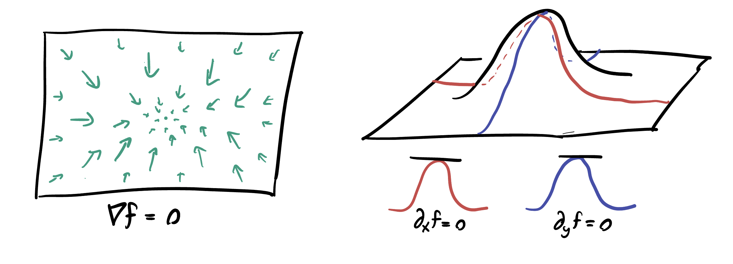
Theorem 11.1 (The Gradient at Extrema) At a local max or min, every directional derivative is zero, because the point is a local max or min in every direction. In particular, all partial derivatives are zero, so the gradient is zero.
Definition 11.2 (Critical Points) The critical points of a function are the points where the gradient is zero.
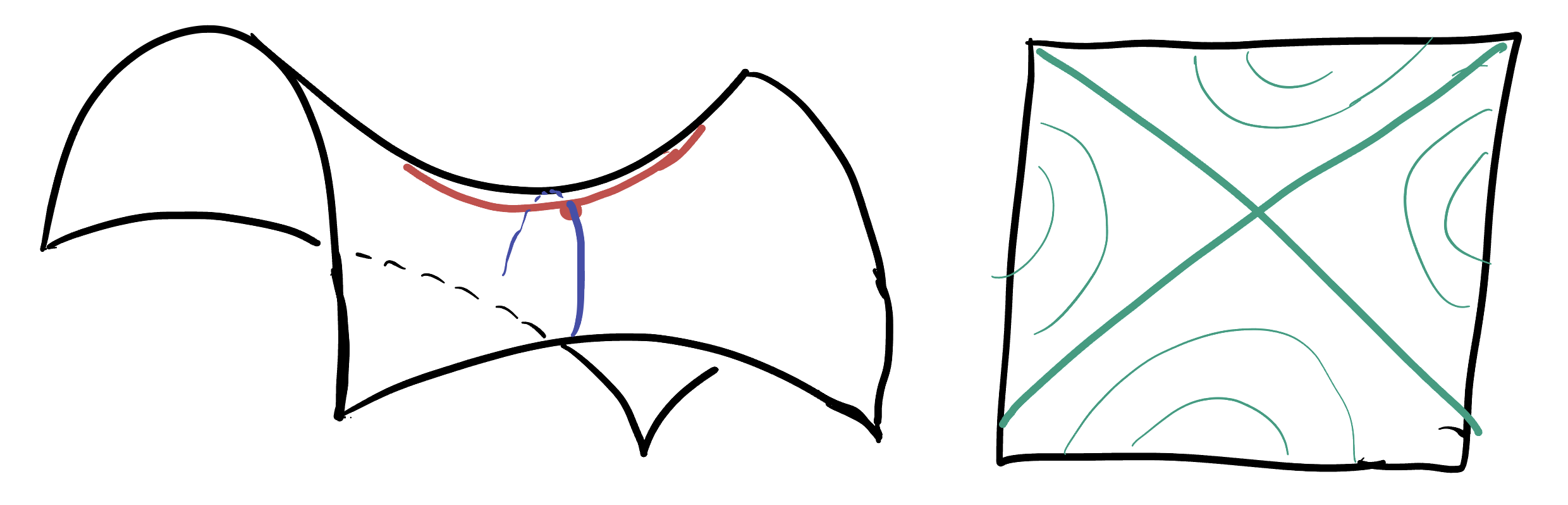
Like in Calculus I, we have to be careful as not all critical points are actually maxima or minima. The standard example there is \(y=x^3\) which has \(y^\prime = 3x^2\) equal to zero at \(x=0\), even though this is not the location of an extremum but rather a point of inflection. Similarly, for multivariable functions the existence of a critical point does not imply the existence of an extremum. The easiest and most common counter-example here is the saddle:
Example 11.1 (Critical Points) Find the critical points of \[f(x,y)=x^3+y^3+6xy\]
Solving the system of equations arising from setting the gradient to zero is the analog of the first derivative test. What’s analog of the second derivative test? In Calculus I, this was looking for the “concavity” of the function, which was simply up or down. But we already know in multiple variables things are more complicated: there are hills, bowls and saddles to contend with.
Our tool to see which is the best local description is the quadratic approximation, which is particularly simple at a critical point. The zeroth order term is just a constant (which shifts a graph up or down but doesn’t affect its shape), and the linear terms are zero - that’s the definition of a critical point! Thus all we are left with are the quadratic terms, which were determined by the Hessian - the matrix of second derivatives.
Here we recall the Hessian, which is a means of organizing all of the second derivative information.
Definition 11.3 (Quadratic Approximation at a Critical Point) Recall the Hessian matrix is the matrix of all second derivatives \[Hf=\pmat{f_{xx}& f_{xy}\\ f_{yx}& f_{yy}}\]
At a critical point, \(p\), up to a constant the quadratic approximation is built out of the Hessian alone
\[f\approx \mathrm{Const}+ \frac{1}{2}\left(f_xx(a,b)(x-a)^2+2f_{xy}(x-a)(y-b)+f_{yy}(a,b)(y-b)^2\right)\] Where here we’ve used that \(f_{xy}=f_{yx}\) to simplify.
To understand if our function has a max, min or saddle at a given critical point, we just need to find a formula in terms of \(f_{xx},f_{xy}\) and \(f_{yy}ee\) that determine the shape of this graph. The important tool here is the determinant (which we already met when computing cross products)
\[D = \det Hf = \det \pmat{f_{xx}& f_{xy}\\ f_{yx}& f_{yy}}= f_{xx}f_{yy}-(f_{xy})^2\]
Where again we’ve used that \(f_{xy}=f_{yx}\) to simplify our formula. The sign of this quantity determines whether the quadratic is a saddle:
Theorem 11.2 If \(p\) is a critical point of \(f(x,y)\) and \(D\) is the determinant of the second derivative matrix at \(p\), then
- \(p\) is a saddle if \(D<0\).
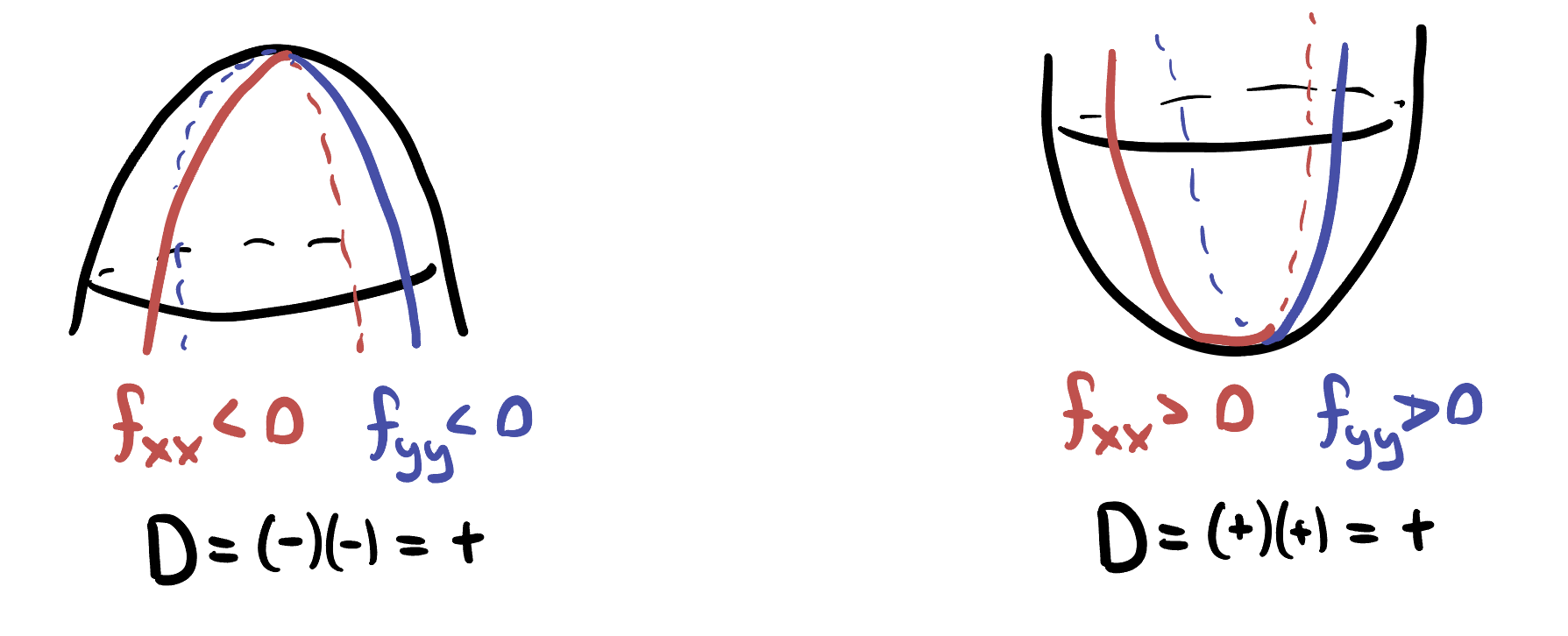
- \(p\) is a minimum if \(D>0\) and \(f_{xx}>0\)
- \(p\) is a maximum if \(D>0\) and \(f_{xx}<0\)
- Otherwise, the test is indeterminant.
It is possible to go beyond the quadratic approximation and understand the points this test labels indeterminant, but this requires more complicated mathematics and rarely shows up in real-world applications.
Its helpful to confirm this test is doing the right thing for examples we already understand: so let’s take a quick look at a maximum, minimum and saddle:

11.1 Finding Maxima Minima and Saddles
Example 11.2 (\(x^2+y^2-2x-6y+14\))
Example 11.3 (\(x^3+y^3+6xy\))
Example 11.4 (\(2x^3-yx+6xy^2\))
11.2 Sketching Multivariate Functions
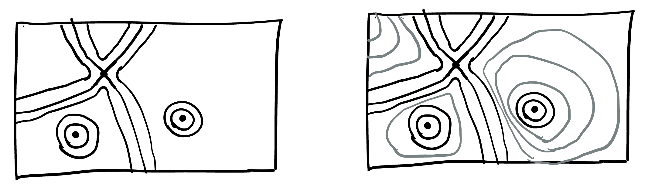
Having precise mathematical tools to understand the critical points of a function allows us to understand the total behavior of the function - because it gives us the tools to draw a contour plot! Here’s an example: say we ran the above computations and found a function with three critical points: a max a min and a saddle.
We plot and label them on an \(xy\) plane, and then we can draw little local models of what the contours must look like nearby, since we know the contours for maxes mins and saddles!

Next, since there are no other critical points we know there isn’t anything else interesting going on in our function’s behavior. So, we can extend this to a drawing of the contour plot for the whole function by first extending the lines that already exist in a way that they do not cross (if they crossed anything else, that would be representing a new saddle- but we know there are none!) And then, we can just fill in contour lines in a non-intersecting way essentially uniquely, so that they create no new saddles or closed loops (which would have a new max or min in their center!)
The observation that makes this possible is that nothing strange can happen away from a critical point: if the first derivative is nonzero, then the function is simply increasing or decreasing (in some direction), and the level sets nearby locally look like a set of parallel lines! This is a gateway to a huge amount of modern and advanced mathematics called morse theory
This technique remains important even beyond scalar functions, where changes in contours signify changes in the topology of a shape!
11.3 Videos
11.3.1 Calculus Blue
11.3.2 Khan Academy
Example Problem: