Assignment 9
Problems
Realistic Optimization
On the last assignment, you helped an engineering team for the NASA Artemis moon mission optimize the width and slope of their rocket’s nose cone for aerodynamic efficiency.
However, after a brief celebration you receive news back from the manufacturing team: your solution simply will not work! While it certainly is the most efficient with regard to air friction, the nose cone is but one piece of a very large and complicated rocket, and there’s other constraints that need to be taken into account.
Indeed, there is a fixed cap on the total weight of the rocket overall, and a fixed percentage of that can be used on materials in the manufacture of the nose cone. You are allotted 800kg of material from which to design the nose cone, and asked to produce a design weighing at most this much.
The original nosecone design violates this, and indeed the team at NASA suggests that you throw out the entire model entirely and re-design the nosecone using lighter-weight specifications. Your new model has a different dependency of thrust on radius and efficiency:
\[F(r,s)=4-r^2-s^2+3rs\]
With this new model, you go back to your modeling software and ask the computer to estimate the weight of a nose cone with radius \(r\) and slope \(s\): it tells you that the weight can be modeled by
\[W(r,s)=100(s^2+r^2)\] (where we require that \(r> 0\) and \(s\geq 0\) as they are a distance and a slope)
Given this thrust equation and weight constraint, what should you bring back to the manufacturing team as the best \((r,s)\) parameters for aerodynamic flight?
The Mass of Steel Sheets
Integrals measure the area under a curve, but appear in a much wider context than simply geometry: often this area is encoding the total amount of some physical property distributed along an interval, rectangle or surface.
One common example is mass: if you have an object of a given fixed density \(\rho\) and volume \(V\), its possible to find the mass as just the density times volume. But if you have an object whose density varies, then the total mass is the integral of its density! This may be familiar already in one dimension from Calc I/II or introductory physics/engineering, where the mass of a 1-dimensional rod from \(x=a\) to \(x=b\) is given by \[m=\int_a^b \rho(x)dx\]
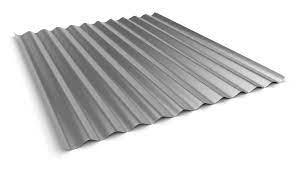
Multivariate integrals bring these techniques much closer to real world application, as real-world objects are often much more than lines! In this problem we will learn how to calculate the mass of a corrugated steel sheet, the kind used in many manufacturing and engineering designs due to its good ratio of strength to weight.

The density of a flat steel sheet is constant (at 2mm thick, its 15kg per square meter). However, a corrugated sheet has a non-constant density across its surface, due to the fact that it bends in one direction (and there is more sheet, hence more steel, in the bends). The density (in kilograms / square meter) of a corrugated sheet is well modeled by the simple expression \[\rho(x,y)=15+0.5\sin^2(5\pi x)\] (The variable \(y\) does not show up in the formula as the sheet is only corrugated in one direction).

You are on a construction team that is looking to plate the outside of a new building in corrugated steel sheets. You are told that a single panel of such sheeting is a rectangle running from \(x=0\) to \(x=3\) meters, and \(y=0\) to \(y=5\) meters.
- Set up a double integral that gives the mass of this sheet. How much does it weigh?
- The building you are looking to cover in panels has an outside surface area of 800 square meters. How many panels do you need to order to complete the project? If each truck bringing in panels has a maximum capacity of one ton (1,000kg) how many truck loads will be required on construction day?
Solutions
Realistic Optimization
In this optimization problem we are confronted with an inequality: we need to make the best rocket nosecone that weights 800 kg or less.
Thus, we need to compare two different optimizations:
- Use unconstrained optimization to find the local maxes and mins of efficiency. Only keep the relevant ones (that is, discard any maxes or mins where \(r,s\) are not positive, or the total mass is greater than 800kg)
- Use constrained optimization to find the maximum values of efficiency directly along the constraint \(w=800\): again, only considering those that are physically relevant (so \(r,s\) must be positive).
Then the true maximum is the largest of the relevant maxima found in these two approaches. We carry them out one at a time below.
Unconstrained Optimization:
We need to compute the first derivatives \(f_r\) and \(f_s\): setting them equal to zero gives our critical points:
\[f_r=-2r+3s\hspace{1cm}f_s=-2s+3r\]
Setting the second of these to zero says that \(3r=2s\), or \(s=\frac{3}{2} r\). Plugging this into the first, we see \[-2r+3s=0\implies -2r+3\left(\frac{3}{2}r\right)=0\implies \frac{5}{2}r=0\]
Thus \(r=0\). But substituting this back into the second we see \(s=0\), so we have just one critical point \((r,s)=(0,0)\). We could go on to do the second derivative test and figure out if its a max min or saddle (it’s a saddle) but we don’t need to: this isn’t a realistic value for our rocket design! We only care about values where \(r\) and \(s\) are positive, so we can just ignore this one.
Thus, there are no interesting critical points with weight less than 800kg so its time to investigate the configurations with weight exactly 800kg.
Constrained Optimization:
To deal with the constraint \(W=800\), we use lagrange multipliers. To make some numbers a little better, we can divide both sides of the constraint by 100 to get \[r^2+s^2=8\]
We already have the gradient of \(f\) from the previous part \(\nabla f =\langle f_r,f_s\rangle\) and using our rescaled constraint \(\nabla w =\langle 2r,2s\rangle\) so the system of equations we want to solve is
\[\left\{ \begin{matrix} -2r+3s=\lambda 2r\\ -2s+3r=\lambda 2s\\ r^2+s^2=8 \end{matrix} \right\}\]
We only care about the values of \(r\) and \(s\) so one approach to solving this is to try and *eliminate \(\lambda\). We can solve for \(\lambda\) in each of the first two equations by dividing by \(r,s\) respectively to get
\[\frac{-2r+3s}{2r}=\lambda=\frac{-2s+3r}{2s}\]
Of course this is only valid if we are allowed to divide by \(r\) and \(s\), so we have two other cases to consider \(r=0\) and \(s=0\). But these aren’t realistic as we only care about positive \(r\) and \(s\) solutions, so we can ignore them from the get-go! (In fact, if you continue the analysis you find that \(r=0\) implies \(s=0\) but the point \((r,s)=(0,0)\) doesn’t satisfy the constraint, so there’s no solution here anyway, and same for \(s=0\)).
Now we need to solve the equation we got from equating each \(\lambda =\cdots\). We can simplify the fractions on each side to give
\[-1+\frac{3s}{2r}=-1+\frac{3r}{2s}\]
Adding 1 to both sides cancels the \(-1\), giving \(3s/2r = 3r/2s\). We can then multiply through by \(2/3\) to cancel the constants, giving
\[\frac{s}{r}=\frac{r}{s}\,\,\implies\,\, s^2=r^2\]
Taking a square root yields that \(r=\pm s\), which we can then substitute into the constraint:
\[r^2+s^2=(\pm s)^2+s^2=2s^2=8\] \[\implies s^2=r\implies s=\pm 2\]
So \(s\) can be either \(2\) or \(-2\), and for every value of \(s\) we can have \(r\) equal to plus or minus this value. This gives four critical points to consider
\[(-2,-2),(-2,2),(2,-2),(2,2)\]
But we are after realistic solutions and require \(r,s\) to both be positive! Thus only one of these is relevant to us, \((r,s)=(2,2)\). This is our optimal solution, with
\[f(2,2)=4-2^2-2^2+3\cdot 2\cdot 2=8\]
The Mass of Steel Sheets
We are given the mass density \(\rho(x,y)=15+0.5\sin^2(5\pi x)\) and the size of the sheet \(x\in[0,3],y\in[0,5]\). So, finding its mass just amounts to calculating a double integral:
\[M=\iint_R \rho dA = \int_0^5\int_0^3 15+\frac{1}{2}\sin^2(5\pi x)\,dx\,dy\]
We evaluate this as an iterated integral, so we can first focus just on the \(x\) integral. This has \(\sin^2\) in it, so we use a trigonometric identity to simplify
\[\sin^2(5\pi x)=\frac{1-\cos 10\pi x}{2}\]
\[\int_0^3 15+\frac{1}{2}\frac{1-\cos (10 pi x)}{2}dx\] \[=\int_0^3 15dx+\int_0^3\frac{1}{4}(1-\cos(10\pi x))dx\] \[= 45+\frac{1}{4}\left(x-\frac{\sin(10\pi x)}{10\pi}\right)\Bigg|_0^3\] \[=45+\frac{1}{4}\left(3-\frac{0}{10\pi}\right)\] \[=45+\frac{3}{4}=45.75\]
Now, we integrate the result with respect to \(y\):
\[M=\int_0^5 45.75dy=45.75*5=228.75\mathrm{kg}\]
The building has a surface area of \(800m^2\) and each panel is \(3\times 5=15m^2\). Thus we need \(800/15= 53.33\ldots\) panels, so in reality we need 54 panels to make sure we can cover it all.
Each truck can carry \(1000kg\) total which is \[\frac{1000}{228.75}=4.37\textrm{ panels}\]
Thus, every truck can carry \(4\) panels (as 5 would be too many for its weight). We need 54 panels total, so the number of truck loads required is
\[\frac{54}{4}=13\]