Extra: Fall Break Optional
Problems
Level Sets & The Gradient
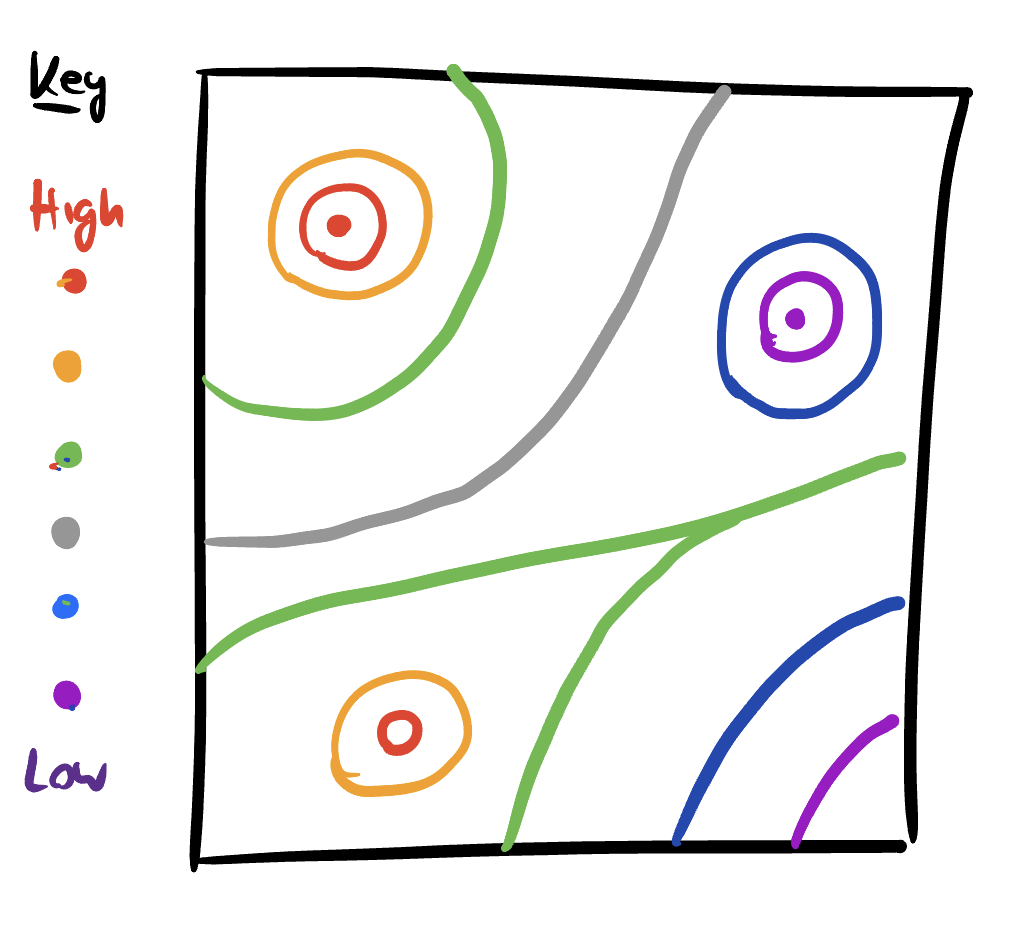
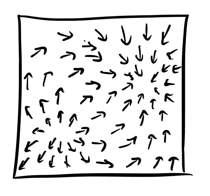
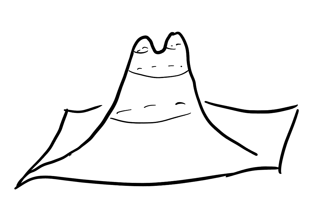
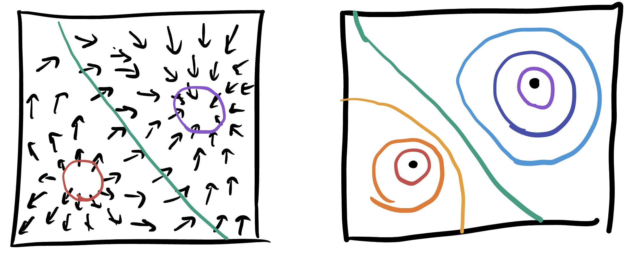
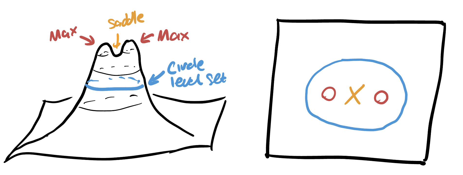
Below are depictions of three functions \(f,g,h\colon\mathbb{R}^2\to\mathbb{R}\). In the first, I have given you a picture of the level curves of \(f(x,y)\). In the second, I have drawn the gradient of \(g\). In the third, I have drawn a graph of \(h\). Your job is to practice translating between these three modalities of understanding a multivariate function.
- Draw a sketch of the gradient of \(f\), and explain in a sentence or two your diagram: why did you draw the arrows you did?
- Draw a sketch of the level sets of \(g\), and explain in a sentence or two your diagram: why did you draw the curves you did?
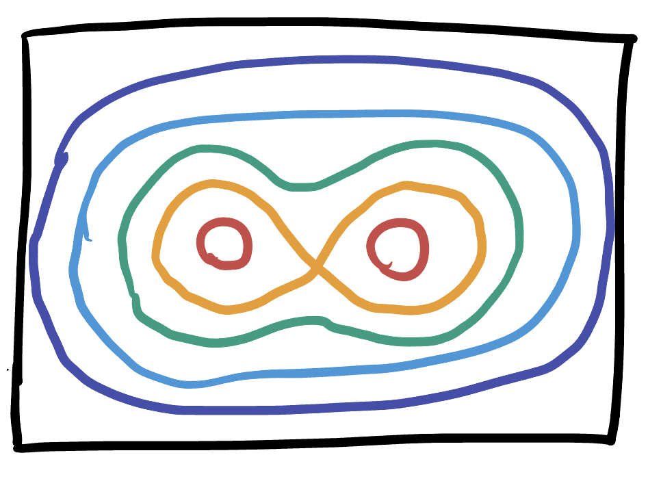
- For \(h\), you can choose: either draw me a diagram of the level sets of \(h\), or the gradient of \(h\). Explain in a sentence why your sketch looks like it does.
Function Sketching
Consider the function \(f\colon \mathbb{R}^2\to\mathbb{R}\) given by the following formula: \[f(x,y)=x^3+y^3-3xy+14\] In this problem, we work to understand \(f\) without any technology: to showcase the power that calculus has brought us.
- Find the critical points of \(f\), and classify these as max, mins or saddles via the second derivative test.
- Use this classification to sketch the level curves of \(f\) like we did in class. Start by drawing the level curves near each max, min and saddle. Then use that level curves cannot cross (away from a saddle) and there are no other max/mins to fill in the rest of the picture.
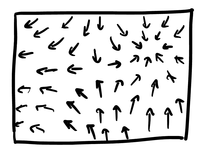
- Use this sketch of the level curves of \(f\) and the information about which points are maxima and minima to sketch the gradient of \(f\).
High Dimensional Optimization
In class we have mainly focused on understanding maxima minima and saddles for functions of two variables. THe main reason for this is just that the computations remain manageable - there are only four second derivatives to deal with, and they all fit nicely into a \(2\times 2\) array. However problems in the real world often have to deal with many many more variables, and this problem is your opportunity to think a bit through how the theory might work here.
Consider you have a function \(f(x_1,\ldots, x_n)\) of \(n\) variables. Such a function has \(n\) first derivatives, so to find its critical points we need to solve a *system of \(n\) equations: this might take some work! But assume that we have such a critical point \(c\), and now we want to know if this is a max, a min or a saddle.
Question: If its a random critical point, what is the probability that its a maximum? Whats the probability is a minimum? A saddle?
Hint: Think about slices! A hill has all of its slices downward shaped parabolas, and a bowl has all of its slices upward facing parabolas, and a saddle is anything else. How many options are there, and how many of them are maxima?*
The answer might surprise you: its rarer than you may think to find a maximum or a minimum in high dimensions! This has implications for optimization in large real world problems like machine learning: you may need to think a little harder to make sure you actually reach a minimum than you’d originally hoped.
Solutions
Level Sets & The Gradient
In this problem the key is to remember the following facts about the gradient:
- The gradient points in the direction of steepest increase of the function
- The gradient is orthogonal to level sets of the function
And the following facts about level sets of a function:
- Near a max or a min, level sets look like concentric circles
- Near a saddle, level sets make an “X” shape.
In the first part of the problem, we are given the level sets and asked to draw the gradient. We automatically know the gradient vectors will be perpendicular to the level sets, and since the level sets come with a legend telling us which ones are high valued and which ones are low, we can see the direction. I started by drawing a couple gradient vectors directly on the level set sketch, and used these as a guide to fill in the rest:
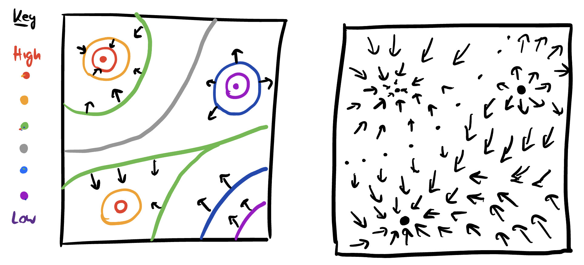
Next we started with a plot of the gradient and needed to draw level sets. First we notice there is one spot where the gradient is pointed inwards, and one spot where its pointed outwards in every direction. Since the gradient always points towards the steepest increase, these are a max and min respectively. And, we know maxes and mins are surrounded by concentric circle level sets. Second, we can see the gradients all point in approximately the same direction across the middle of the image, so the level set there is approximately linear. From this, we can fill in the rest by making sure they never cross (making a saddle) or close up to form any other families of circles (making a new max or min):
Finally we are given a picture of a graph in 3D and told to draw its gradient or its level sets. I’ll draw the level sets: if you want to draw the gradient you can follow the procedure we did above to convert my picture. The first thing we notice is the function graphed has two maxes and a saddle. So, let’s label those and then draw what the nearby level sets look like:
We also see by looking farther down the function that the level sets must eventually become circles, so we add one of these too. Then we can just fill everything in, by making sure the level sets never cross or close off to form more families of circles:
Function Sketching
To sketch the level sets and gradient of this function, we first must find the critical points and classify them. Taking the graident,
\[\nabla f = \langle 3x^2-3y,3y^2-3x\rangle\]
So the system of equations we need to solve is (after dividing by the 3):
\[\left\{x^2=y,\,y^2=x\right\}\]
Substituting the first equation into the second we see
\[y^2=(x^2)^2=x^4=x\]
Thus either \(x=0\) (and hence \(y=0\)) or \(x^3=1\). But this only has the solution \(x=1\) (and hence \(y=1\)), so there are two critical points
\[\{(0,0),(1,1)\}\]
To classify them, we need to apply the second derivative test:
\[f_{xx}=6x\hspace{1cm}f_{xy}=-3\hspace{1cm}f_{yy}=6y\]
Thus the Hessian matrix and its determinant are
\[H=\pmat{6x &-3\\-3&6y}\hspace{1cm}D=\det H=36xy-9\]
Evaluating this at the critical points gives \(D(0,0)=-9\), so \((0,0)\) is a saddle, and \(D(1,1)=36-9=25\), so \((1,1)\) is either a max or min. To figure out we look at the sign of \(f_{xx}\) or \(f_{yy}\). Both of these are positive, so its a minimum.
To sketch the level sets, we can start with the local model of a minimum (concentric rings) at \((1,1)\) and of a saddle (an X shape) at \((0,0)\), then fill in the rest of the plot making sure no other level sets cross or close up into circles.
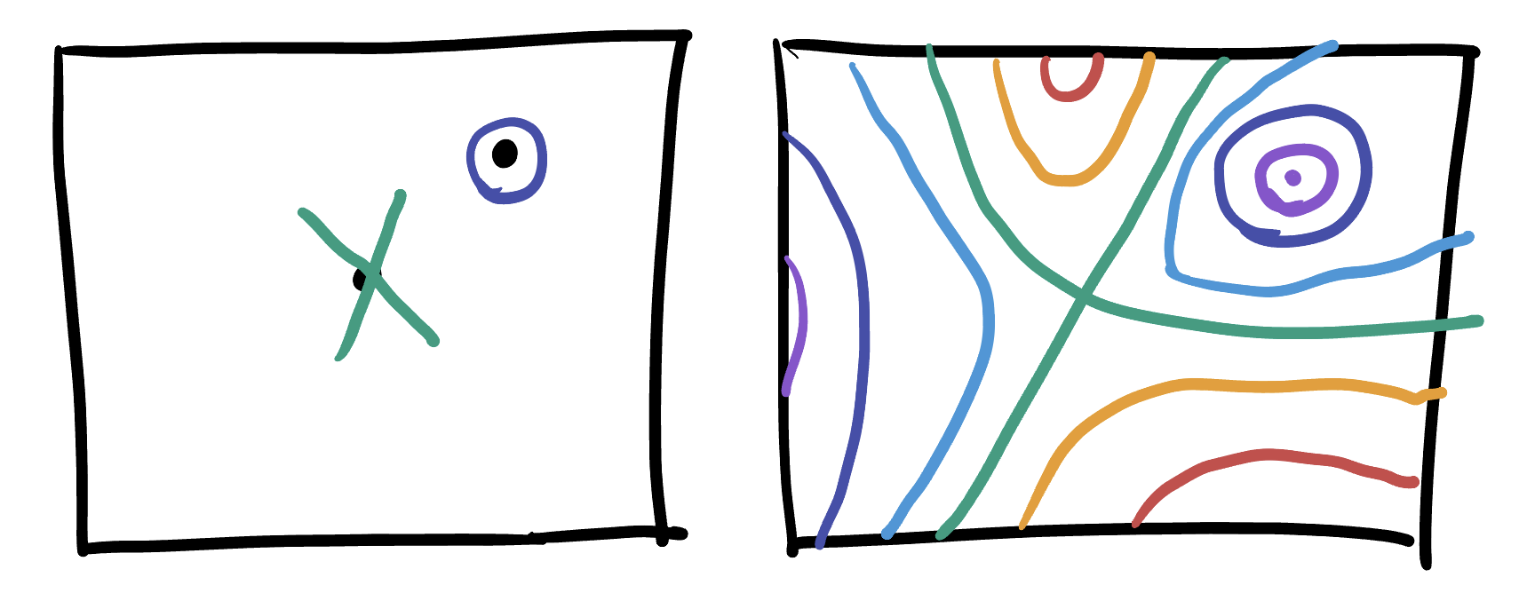
Given this picture, we can draw the gradient by remembering its orthogonal to level sets, and points in the direction of maximum increase. Since we know that saddles go upwards along one axis and downwards along the other, knowing where the minimum is sorts out the directions of everything else:
High Dimensional Optimization
At a critical point, we can imagine computing the quadratic approximation there. Slices of this quadratic approximation are going to be parabolas, some of which are pointing upwards, and some of which are pointed downwards. If we have \(n\) variables, then there are \(n\) different slices (one for each coordinate axis). Let’s try to count these: if each of the \(n\) coordinates can be an upwards or downward parabola, there are two choices for \(n\) things, which means theres \(2\cdot 2\cdots 2=2^n\) possibilities overall.
To get a maximum, we need all of the slices to be downwards. To be a minimum, we need all of the slices to be upwards. And anything else - any combo of upwards and downwards parabolas, is some type of saddle. Thus, the number of saddles is \(2^n-2\) and the probabilities of each type are
\[P_{\max} = \frac{1}{2^n}\hspace{1cm}P_{\min} = \frac{1}{2^n}\hspace{1cm} P_{\mathrm{saddle}}=\frac{2^n-2}{2^n}\]
Even in 10 dimensions this is already pretty surprising: the chance of a random critical point being a max or min is \(0.097\) percent, and the chance of it being a saddle is 99.8 percent.