Assignment 6
Problems
Parameterizing a Tube Around a Curve
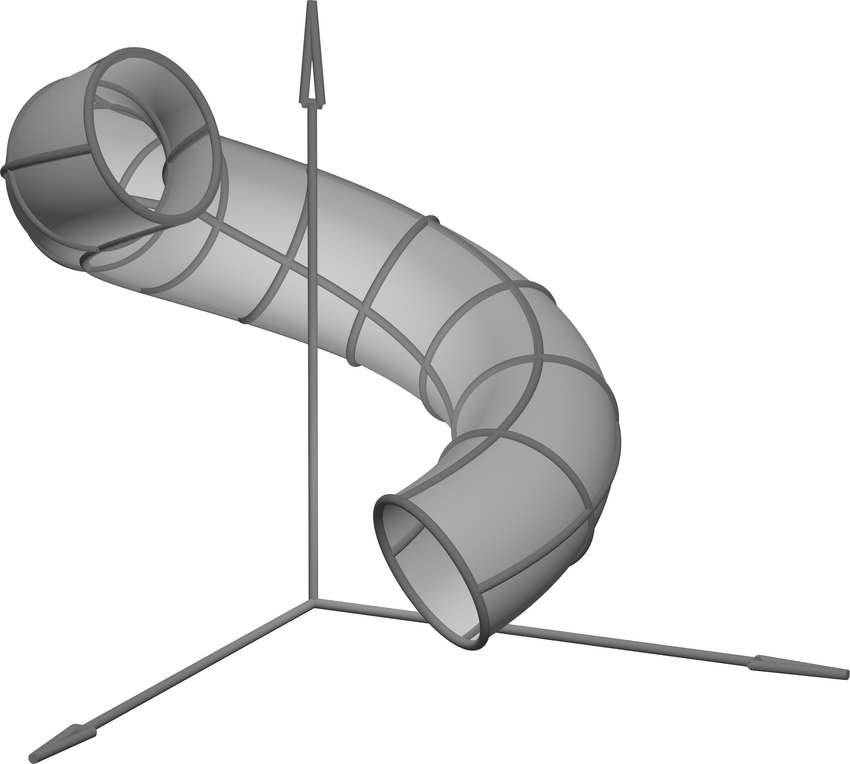
A fundamental task in 3-dimensional computer modeling is to render a three dimensional curve. Every serious software package for 3D modeling has some sort of Tube object one can feed in a parametric curve, and get out a mesh describing a 2-dimensional surface of a tube surrounding that curve of constant radius.
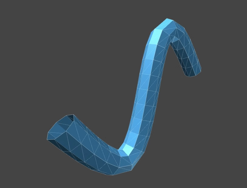
The image above shows the class TubeGeometry() from Three.js, the browser-based 3D graphics engine I use to make animations for our class. In this exercise we work out the theory for doing this, that the authors of such 3D software systems need to code. Then we implement this theory in a specific case (the helix).
The General Theory
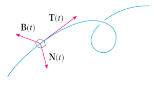
Let \(\vec{r}(t)\) be a parametric curve in 3 dimensional space. Recall from class that at each time \(t\) we can define three vectors based at the point \(\vec{r}(t)\) that are useful in understanding its behavior:
- The unit tangent vector \(\vec{T}(t)=\frac{\vec{r}^\prime(t)}{|\vec{r}^\prime(t)|}\)
- The unit normal vector \(\vec{N}(t)=\frac{\vec{T}^\prime(t)}{|\vec{T}^\prime(t)|}\)
- The unit binormal vector \(\vec{B}(t)=\vec{T}(t)\times \vec{N}(t)\).
To parameterize a tube around a curve, what we really need to be able to do is to draw a circle which is orthogonal to the curve at each point. Then we stitch together these circles for each value of \(t\) to get a solid tube.
To derive a general formula, follow the steps below:
- Explain of the vectors \(T,N,B\) do you need to define an orthogonal plane to the curve \(\vec{r}(t)\) at a point?
- Given any two orthogonal unit vectors \(\vec{v},\vec{w}\), the parametric curve \(\vec{c}(s)=\cos(s)\vec{v}+\sin(s)\vec{w}\) is a circle in a plane parallel to \(\vec{v},\vec{w}\). Use this to write down a circle of radius \(R\) which is orthogonal to our curve at \(\vec{r}(t)\) (the final expression will have a \(t\) for the position along the curve, as well as an \(s\) for the position along the circle).
- The circle you’ve constructed is centered at \((0,0,0)\). Translate it by \(\vec{r}(t)\) to put its center on the curve instead. This gives a final formula in \(s\) and \(t\) the orthogonal circles to the curve which determine the tube!
In a computer, we often program this general formula and then when the user inputs a curve \(\vec{r}(t)\), the computer computes \(T,N,B\) using calculus, and then finds the tube using the parameterization you just wrote down. But for practice, let’s do just one example by hand.
A spring shaped tube: Consider the parametric curve for a helix \[\vec{h}(t)=(\cos t,\sin t,t)\]
- Compute \(T,N,B\) for the Helix
- Use these to write down an equation for a tube around the helix of radius \(1/10\), as a function of \(s\) and \(t\).
Contour Plots
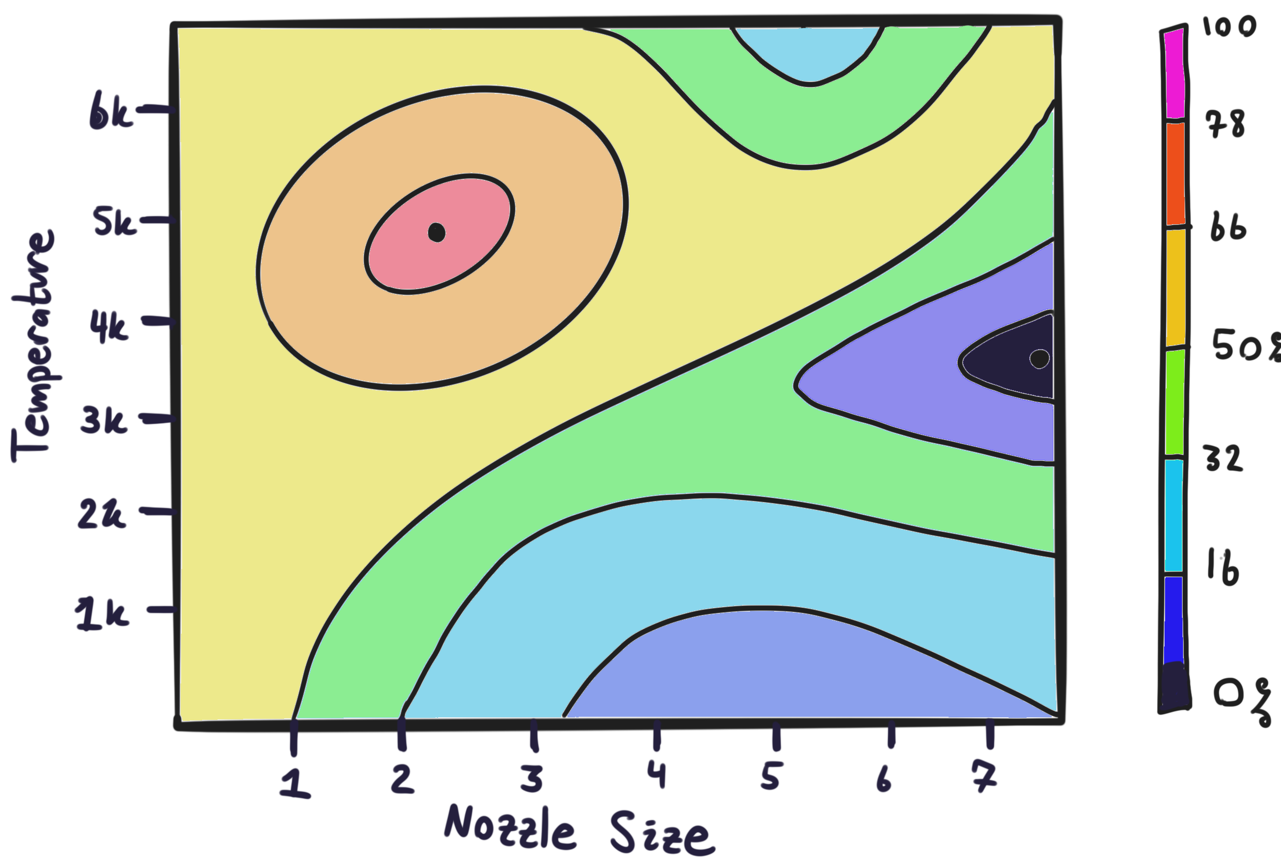
You are hired as a consultant for an aerospace company that is working to design the next generation of rocket boosters. The main goal of your team is to improve the of the engine (the total impulse delivered per kilogram of fuel). You begin by focusing on the two most important variables: the rocket engine nozzle size \(n_s\), and the temperature \(T\) of the burning fuel. You write a computer program to simulate thousands of different combinations of temperature and size, and compute the efficiency \(E_{ff}(T,n_s)\) of each configuration. After a lot of computation, your program outputs the following figure:
How do you summarize your findings to your boss, given this data? An example summary might sound something like this (though this is not the answer for this exact plot, of course!)
For the most part, rocket engines perform better when the nozzle size is large and the temperature is small, though if the temperature gets too low it starts performing worse again. Performance is particularly bad for temperature of 300 and small nozzle sizes (around 1). The most efficient configuration is nozzle=5 and temp=3.2k.
If the current rocket engines in production have a nozzle size of 1 and a fuel temperature of 6k, what concrete suggestion could you make to your team on how to change the design slightly to improve efficiency? What would you say to a team currently building a rocket with nozzle size 7 and temperature 3k?
Example questions you may want to consider: Should you increase both temp and nozzle size? Decrease one of them and leave the other constant?Decrease both? Should they make big or small changes to their current design? Etc….
Derivatives and Multiple Variables
The data of multivariate functions can be presented to us in multiple ways. Sometimes, we are given a contour plot - for example, as the output of a simulation like in the problem above. But other times we are just given an equation, and have to work with that.
In this problem we will continue our roll as an aerospace consultant engineer, working on the same rocket design as above. After successfully helping with the engine design, you are asked to work closer with the team that is building the rocket’s body so that you can safely integrate the engine. This team is run by a collection of theorists who have been able to work out a model for the rocket’s aerodynamic efficiency in terms of the angle \(\alpha\) and height \(h\) of its fins, the radius \(r\) of the main tube, and the thickness \(t\) of the metal support beams. Their model is
\[E = re^{-r/2}\sin(h \alpha / t)\]
Because of your success in optimizing the engine design, this team asks you for your help in optimizing the rocket body. In particular, they are currently considering building a rocket body with radius \(1.5\), beam thickness of \(0.3\), fin angle of \(\pi/4\) and fin height of \(1\).
They want to know should they increase or decrease the beam thickness, to improve efficiency? Because the rocket body design depends on so many parameters, we cant draw its graph (which lives in 5 dimensional space) or its contour plot (which lives in four dimensions!). So, we need to just do some calculus.
Solutions
Parametrizing a Tube.
For deriving the general formula: the tangent vector \(\vec{T}\)(t)$ is tangent to the curve, and the vectors \(N\) and \(B\) are both orthogonal to the curve. Thus, the vectors \(\vec{N}\) and \(\vec{B}\) describe the orthogonal plane to \(\vec{r}(t)\) at any point.
Because the vectors \(\vec{N}(t)\) and \(\vec{B}(t)\) are both unit length and orthogonal to one another, we can define a unit circle in the \(NB\) plane by \(\cos(s)\vec{N}(t)+\sin(s)\vec{B}(t)\). To make a circle of radius \(R\) we simply multiply this equation by \(R\): \[\vec{c}(s)=R\cos(s)\vec{N}(t)+R\sin(s)\vec{B}(t)\] Now all that remains is to translate the circle to be centered at \(\vec{r}(t)\), giving the equation of our tube
\[\begin{align*} \mathrm{tube}(s,t)&=\vec{r}(t)+\vec{c}(s)\\ &=\vec{r}(t)+R\cos(s)\vec{N}(t)+R\sin(s)\vec{B}(t) \end{align*}\]
Now we make this concrete for the helix curve \(\vec{r}(t)=(\cos(t),\sin(t),t)\). Computing the necessary quantities (I’ve left out some of the algebra but you should be showing your work!)
\[\vec{T}(t)=\frac{\vec{r}^\prime(t)}{|\vec{r}^\prime(t)|}=\langle\frac{-\sin t}{\sqrt{2}},\frac{\cos t}{\sqrt{2}},\frac{1}{\sqrt{2}} \rangle\] \[\vec{N}(t)= \frac{\vec{T}^\prime(t)}{|\vec{T}^\prime(t)|}=\langle -\cos t, -\sin t,0\rangle\] \[\vec{B}{t}=\vec{T}(t)\times \vec{N}(t)=\left|\begin{matrix}\hat{i}&\hat{j}&\hat{k}\\ \frac{-\sin t}{\sqrt{2}} & \frac{\cos t}{\sqrt{2}} &\frac{1}{\sqrt{2}}\\ -\cos t & -\sin t &0\ \end{matrix}\right|= \langle\frac{\sin t}{\sqrt{2}},\frac{-\cos t}{\sqrt{2}},\frac{1}{\sqrt{2}} \rangle\]
With the radius \(R=1/10\), we can just plug everything into our formula and simplify:
\[\begin{align*} \mathrm{tube}(s,t)&=\vec{r}(t)+\frac{\cos s}{10}\vec{N}(t)+\frac{\sin s}{10}\vec{B}(t)\\ &=(\cos(t),\sin(t),t)+\frac{\cos s}{10}\langle -\cos t, -\sin t,0\rangle + \frac{\sin s}{10}\langle\frac{\sin t}{\sqrt{2}},\frac{-\cos t}{\sqrt{2}},\frac{1}{\sqrt{2}} \rangle\\ &=\left\langle \cos t -\frac{\cos s\cos t}{10}+\frac{\sin s\sin t}{10\sqrt{2}},\sin(t)-\frac{\cos s\sin t}{10}-\frac{\sin s\cos t}{10\sqrt{2}},t+\frac{\sin s}{10\sqrt{2}} \right\rangle \end{align*}\]
Reading Contour Plots
This plot shows that rocket engine efficiency is maximized around a nozzle size of 2, and a temperature of 5k. Small changes from this configuration in any way decrease the efficiency somewhat. The worst performing rocket engines are those with large nozzle size, and temperature around mid-range (3k degrees).
If the team is currently building a rocket with nozzle size 1 and temperature 6k, they should slightly decrease the temperature while increasing nozzle size, in order to best increase efficiency.
Partial Derivatives
A function is increasing if its derivative is positive, and decreasing when the derivative is negative. Here we want to know if the efficiency is increasing or decreasing as we change the beam thickness, so we need to take the partial derivative in the direction of the variable \(t\).
Computing this,
\[\partial_t E=\partial_t\left(re^{r/2}\sin\left(\frac{h\alpha}{t}\right)\right)=re^{-r/2}\cos\left(\frac{h\alpha}{t}\right)\left(\frac{-h\alpha}{t^2}\right)\]
Next, because we are only interested in what is happening near the actual rocket configuration being built, we must plug in the current rocket parameters of \(r=1.5, t=0.3\) and \(\alpha=\pi/4\) to get
\[\begin{align*}\partial_t E&=1.5 e^{-0.75}\cos\left(\frac{(1)(\pi/4)}{0.3}\right)\left(\frac{-(1)(\pi/4)}{0.3^2}\right)\\ &=0.70854\cdot (-0.8660)\cdot (-8.7266)\\ &=5.354603 \end{align*}\]
This is positive, so we should increase thickness if we want to improve the efficiency of our current rocket design.