Chapter 10

Scalar Fields, Graphs, and Level Sets

Part II studied functions whose input was one parameter and whose output was a point or vector. We now reverse that arrangement:

c u r v e : ℝ \to ℝ 𝑛, s c a l a r f i e l d : 𝐷 \subseteq ℝ 𝑛 \to ℝ .

A scalar field takes a point with several coordinates and returns one number.

10.1Scalar Fields

So far in this course we have been studying parametric curves. These are functions which have a single input (the parameter) and multiple outputs (perhaps $𝑥, 𝑦, 𝑧$ or a color for each pixel of an image, etc.) Now we turn to reverse the situation, a function which has multiple inputs but a single output! These are sometimes called multivariable functions (to emphasize the number of inputs), but also are called scalar functions (to emphasize the output is a single number, or a scalar).

In physics, functions with multiple inputs are often called fields. So yet another name for this class of things is a scalar field! We will use scalar field as our default term, while remembering that multivariable function and scalar-valued function describe the same objects.

Definition 10.1 (Scalar Field). A scalar field is a function

𝑓 : 𝐷 \subseteq ℝ 𝑛 \to ℝ

which takes in an $𝑛$ -tuple of real numbers and outputs a single real number.

Such a function is written $𝑓 (𝑥, 𝑦, 𝑧, \dots)$ ; for example,

𝑓 (𝑥, 𝑦, 𝑧) = 2 𝑥 2 - 3 𝑥 + s i n (𝑒 𝑧) .

The domain of a scalar field is the set of inputs for which the function makes sense.

Example 10.2. The domain of $𝑓 (𝑥, 𝑦) = l n (𝑥 2 + 𝑦 2 - 1)$ is the exterior of the unit circle in the plane, $𝐷 = {(𝑥, 𝑦) ∣ 𝑥 2 + 𝑦 2 > 1}$ . This is because the logarithm of zero or a negative number is undefined, so the allowable inputs are precisely those for which $𝑥 2 + 𝑦 2 - 1$ is positive.

Our goal in this chapter is to get comfortable with scalar fields from two different perspectives: drawing graphs and drawing level sets.

Scalar fields show up everywhere in mathematics and the sciences. Consider the temperature in a room: this is a function that takes in a point (say, with three coordinates $(𝑥, 𝑦, 𝑧)$ ) and returns a single number - the temperature of the air at that point in space. This is then a function $𝑇 : ℝ 3 \to ℝ$ .

If we wanted to track the temperature over time, this could be done with a function $ℝ 4 \to ℝ$ which takes $(𝑥, 𝑦, 𝑧, 𝑡)$ and returns the temperature there.

Of course - temperature is just an arbitrary (but conceptually useful!) example. Any quantity you can measure at different points in space(time) gives a scalar function of 3 or 4 variables!

Figure 10.1 Drag the probe: wherever you put it, the plate has a temperature there, and the figure reports the one number. The color is not decoration—it is that same number at every point at once, which is what a scalar field is. Nothing changes if the plate is replaced by a room and the input becomes

(𝑥, 𝑦, 𝑧)

, or by a room over an afternoon and the input becomes

(𝑥, 𝑦, 𝑧, 𝑡)

; only the number of inputs grows, and the single output stays a single output.

Exercise 10.3. Come up with some examples of scalar functions that you think about in daily life (without necessarily having ever thought about them mathematically!)

10.2Graphs and Slices

The graph of a 1-variable function $𝑓$ is a curve in the plane: it is the set of points $(𝑥, 𝑦)$ where $𝑦 = 𝑓 (𝑥)$ . We can make a similar definition for the graph of a scalar field.

Definition 10.4 (Graph of a Scalar Field). The graph of a function $𝑓 : 𝐷 \subseteq ℝ 𝑛 \to ℝ$ is the subset of $ℝ 𝑛 + 1$ given by

g r a p h (𝑓) = {(⃗ 𝑥, 𝑓 (⃗ 𝑥)) : ⃗ 𝑥 \in 𝐷} .

This isn't that useful for visualizing unless dimensions are pretty small! If there are $𝑛$ inputs and $1$ output we need $𝑛 + 1$ dimensions to put them all on a graph. And, if we want to actually see the graph it better fit inside of 3D space so $𝑛$ can only be 1 (the case we already know!) or $2$ .

If $𝑛 = 2$ , then we have two input variables and it is easiest to think of them as being on the $𝑥 𝑦$ plane. Then we may name the output variable $𝑧$ , and plot our function $𝑧 = 𝑓 (𝑥, 𝑦)$ as the points $(𝑥, 𝑦, 𝑓 (𝑥, 𝑦))$ in 3D space.

Drawing a 3D graph is difficult to do in general: but often we can use our knowledge of 2D graphs to try and build up an understanding by slicing. The idea is to take a function $𝑧 = 𝑓 (𝑥, 𝑦)$ and plug in constant values for one of the variables, then try to stack these slices to get a model of the entire surface.

Example 10.5 (Slicing $z=x^2+y^2$). Slices of this function are parabolas in both the $𝑥$ and $𝑦$ directions. Fixing $𝑦$ equal to different values, the parabolas shift upwards! For $𝑦 = 0, 1, 2$ we get

𝑧 = 𝑥 2, 𝑧 = 𝑥 2 + 1 𝑧 = 𝑥 2 + 4

Figure 10.2 Hold one variable fixed and a surface becomes a curve you already know how to read. The cutting plane is drawn in the color of the axis it is perpendicular to, and the curve it leaves behind is plotted beside it as an ordinary graph in the variable that survived. Stack the slices to see the surface as a family of them: for the bowl every slice is a parabola, and it is the way they shift that makes the surface.

There are a couple multivariable functions whose graphs are good to know. Indeed - we've already met some of these before! If $𝑓 (𝑥, 𝑦)$ is a linear equation like $𝑎 𝑥 + 𝑏 𝑦 + 𝑐$ , the graph is the set of points

𝑧 = 𝑎 𝑥 + 𝑏 𝑦 + 𝑐

This is a plane! (It might help to rewrite as $𝑎 𝑥 + 𝑏 𝑦 - 𝑧 = - 𝑐$ to see it is an implicit equation, with normal vector $⟨ 𝑎, 𝑏, - 1 ⟩$ .)

What about $𝑧 = 𝑥 2 + 𝑦 2$ ? We saw this one above in our discussion of slicing, and we also saw it earlier in our study of standard surfaces: it is a circular paraboloid!

Another useful function to know is the saddle surface $𝑧 = 𝑥 2 - 𝑦 2$ . We also met this one back in the discussion of standard surfaces.

Vertical slices fix $𝑥$ or $𝑦$ and leave an ordinary graph. We can also slice the graph with a horizontal plane $𝑧 = 𝑐$ . Those horizontal slices lead to our second way of seeing a scalar field.

10.3Level Sets and Contour Plots

Above we looked at one means of drawing a graph by slicing: we attempted to slice it by vertical planes into the graphs of simpler 1-dimensional functions that we already knew! This works sometimes, but if you can't quickly stack the slices into a coherent image in your mind, knowing the slices won't help you with much else.

So here, we seek other methods of understanding these functions, beyond their graphs. By far the most useful way to depict multivariable functions is by instead slicing with horizontal planes and drawing their level sets.

Definition 10.6 (Level Set). For a scalar field $𝑓 : 𝐷 \subseteq ℝ 𝑛 \to ℝ$ and a number $𝑐 \in ℝ$ , the level set corresponding to $𝑐$ is

𝐿 𝑐 = {⃗ 𝑥 \in 𝐷 : 𝑓 (⃗ 𝑥) = 𝑐} .

For a function of two variables, a level set is commonly a curve in the plane; for a function of three variables, it is commonly a surface in space. A level set can also be empty, consist of isolated points, or have a singularity.

I often think about "sea level" when I think of a level set - a coastline is the level set $ℎ (𝑥, 𝑦) = 0$ above the water. And different level sets correspond to what the coastlines would be if the sea was at different heights.

Figure 10.3 Raise the sea and watch the coastline move. One position of the sea gives one level set

𝐿 𝑐 = {(𝑥, 𝑦) : ℎ (𝑥, 𝑦) = 𝑐}

—a single curve in the plane, and nothing else. Switch to the contour plot and every level is drawn at once, which is why a map tells you the shape of a landscape you have never seen. Where the curves crowd together the hillside is steep; where they spread apart it is gentle. Two distinct levels never cross, because a point has only one elevation.

A contour plot is a drawing of the domain of a function, with level sets representing various values of the range. These are perhaps most familiar from elevation maps. Drawing multiple level sets at once gives a good sense of the behavior of the entire function, though it is most effective when the individual level sets are labeled somehow (often by color) so you can get a sense of their relative values.

A single level set of a function is actually something that you've encountered in previous courses: we called it an implicit equation as it defines a shape implicitly by saying $(𝑥, 𝑦)$ lives on the curve if $ℎ (𝑥, 𝑦)$ has a specific value - instead of specifying it explicitly like a function.

The relationship between the graph and its level sets is particularly direct: intersect the graph $𝑧 = 𝑓 (𝑥, 𝑦)$ with the horizontal plane $𝑧 = 𝑐$ , then project that intersection down to the $𝑥 𝑦$ plane.

Figure 10.4 Where the horizontal plane

𝑧 = 𝑐

meets the graph is a curve at height

𝑐

; drop it straight down and it lands in the domain as the level set

𝐿 𝑐

. That fall is the whole relationship between the two pictures. Slide

𝑐

and watch a level set of the bowl shrink to a point and then vanish—a level set is allowed to be empty—while the saddle's zero level crosses itself at the saddle point.

After looking at several functions and their level sets, you'll start to notice that there are a couple "important behaviors" that show up again and again. These are

Concentric rings around a point
Nearly parallel lines
A level curve crossing itself

These signify three important types of behavior, which we can see by looking back to our useful graphs to know.

Concentric rings around a point often signify the function has either a maximum or a minimum there.

Nearly parallel lines describe a regular region where the function is increasing or decreasing.

A level curve crossing itself commonly means that we are at a saddle shaped point on our graph - it increases in some directions and decreases in others.

These are useful common patterns, but they are not a complete classification of everything a level set can do.

Figure 10.5 Three common things a contour map can do near a point. Drag the lens: almost everywhere the curves look like parallel lines, and the function is simply going uphill. Closed loops nesting inward often mark a peak or a basin. A level curve crossing itself commonly marks a saddle, where the function rises in one direction and falls in another. The last two patterns often draw our attention to points where the gradient vanishes, which is what makes those points worth hunting for in Chapter 14.

Distinct level sets cannot cross: if a point belonged to both $𝐿 𝑐$ and $𝐿 𝑑$ , then the function would have to take both values $𝑐$ and $𝑑$ at that point. A single level set can cross itself, however, as the zero level of $𝑓 (𝑥, 𝑦) = 𝑥 2 - 𝑦 2$ does at the origin.

Functions of three or more variables. Drawing a contour plot is a form of dimension reduction: we've managed to understand the behavior of a function $𝑓$ whose graph $𝑧 = 𝑓 (𝑥, 𝑦)$ lies in 3 dimensional space, by only looking at a 2-dimensional image (its domain, covered in level sets).

This technique can help us level up our intuition to functions of three variables: things like $𝑤 = 𝑓 (𝑥, 𝑦, 𝑧)$ whose graphs would naturally live in four dimensional space!

Exercise 10.7. What do the level sets of the function $𝑤 = 𝑥 2 + 𝑦 2 + 𝑧 2$ look like, for different values of $𝑤$ ?

In three dimensions there are more types of basic behavior than the ones we saw in 2D. You don't need to learn all of them: but to try and get some intuition for the fourth dimension it is a good exercise to try and imagine what the graphs of these functions must be like from their level surfaces.

Figure 10.6 For a function of three variables the graph is out of reach—it would need a fourth dimension—but the level sets are not: they are surfaces sitting in the room with you. Slide

𝑐

through the spheres and they grow; through

𝑥 2 + 𝑦 2 - 𝑧 2

and a two-sheeted hyperboloid pinches into a cone at

𝑐 = 0

and opens the other way. The gyroid is the level set

𝑐 = 0

of a single line of trigonometry, and it divides space into two interlocking halves.

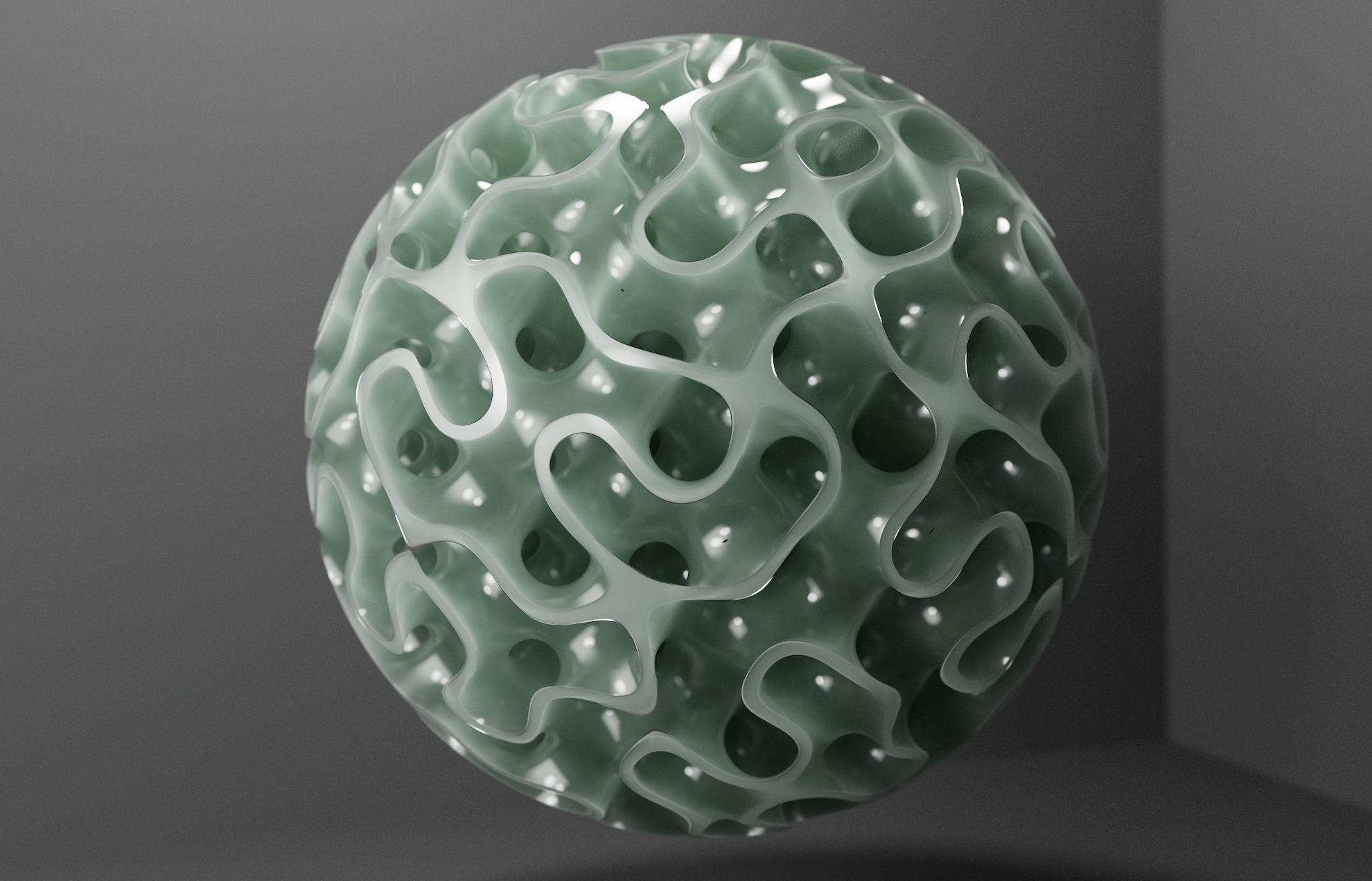
Three dimensional level sets describe implicit surfaces which are extremely useful objects. As we've already seen with curves, sometimes writing down a parameterization can be hard. And this is even more true for surfaces! So having another way to express complicated ones can be a huge help. Below are two examples where I have used implicit surfaces in mathematical rendering.

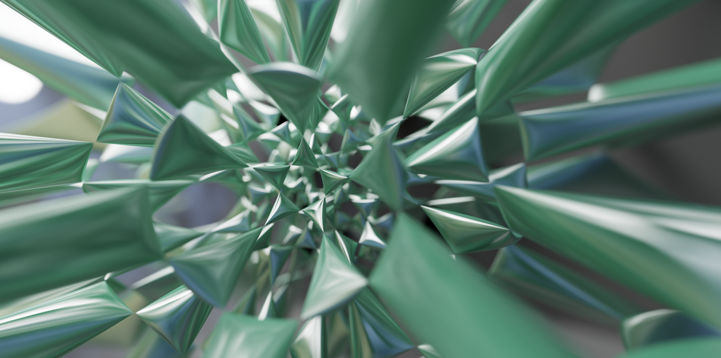
$The gyroid is approximated by the implicit surface \sin(x)\cos(y)+\sin(y)\cos(z)+\sin(z)\cos(x)=0.$

This next surface is called the Barth decic and arises in a field of mathematics called algebraic geometry. Let

𝜙 = 1 + \sqrt 5 2

be the golden ratio. The scale- $1$ surface pictured below is defined by

8 (𝑥 2 - 𝜙 4 𝑦 2) (𝑦 2 - 𝜙 4 𝑧 2) (𝑧 2 - 𝜙 4 𝑥 2) \cdot (𝑥 4 + 𝑦 4 + 𝑧 4 - 2 𝑥 2 𝑦 2 - 2 𝑥 2 𝑧 2 - 2 𝑦 2 𝑧 2) + (3 + 5 𝜙) (𝑥 2 + 𝑦 2 + 𝑧 2 - 1) 2 (𝑥 2 + 𝑦 2 + 𝑧 2 - (2 - 𝜙)) 2 = 0 .

The Barth decic.

The graph of a scalar field may require one dimension too many to see, but its level sets remain in the input space. In the next chapter, we begin measuring how the field changes there by differentiating one input direction at a time.